
Image clustering with Keras and k-Means
A while ago, I wrote two blogposts about image classification with Keras and about how to use your own models or pretrained models for predictions and using LIME to explain to predictions.
Recently, I came across this blogpost on using Keras to extract learned features from models and use those to cluster images. It is written in Python, though - so I adapted the code to R. You find the results below.
One use-case for image clustering could be that it can make labelling images easier because - ideally - the clusters would pre-sort your images, so that you only need to go over them quickly and check that they make sense.
Libraries
Okay, let’s get started by loading the packages we need.
library(keras)
library(magick)  # for preprocessing images
library(tidyverse)
library(imager)
Pretrained model
And we load the VGG16 pretrained model but we exclude the laste layers.
model <- application_vgg16(weights = "imagenet",
                           include_top = FALSE)
model
## Model
## ___________________________________________________________________________
## Layer (type) Output Shape Param #
## ===========================================================================
## input_1 (InputLayer) (None, None, None, 3) 0
## ___________________________________________________________________________
## block1_conv1 (Conv2D) (None, None, None, 64) 1792
## ___________________________________________________________________________
## block1_conv2 (Conv2D) (None, None, None, 64) 36928
## ___________________________________________________________________________
## block1_pool (MaxPooling2D) (None, None, None, 64) 0
## ___________________________________________________________________________
## block2_conv1 (Conv2D) (None, None, None, 128) 73856
## ___________________________________________________________________________
## block2_conv2 (Conv2D) (None, None, None, 128) 147584
## ___________________________________________________________________________
## block2_pool (MaxPooling2D) (None, None, None, 128) 0
## ___________________________________________________________________________
## block3_conv1 (Conv2D) (None, None, None, 256) 295168
## ___________________________________________________________________________
## block3_conv2 (Conv2D) (None, None, None, 256) 590080
## ___________________________________________________________________________
## block3_conv3 (Conv2D) (None, None, None, 256) 590080
## ___________________________________________________________________________
## block3_pool (MaxPooling2D) (None, None, None, 256) 0
## ___________________________________________________________________________
## block4_conv1 (Conv2D) (None, None, None, 512) 1180160
## ___________________________________________________________________________
## block4_conv2 (Conv2D) (None, None, None, 512) 2359808
## ___________________________________________________________________________
## block4_conv3 (Conv2D) (None, None, None, 512) 2359808
## ___________________________________________________________________________
## block4_pool (MaxPooling2D) (None, None, None, 512) 0
## ___________________________________________________________________________
## block5_conv1 (Conv2D) (None, None, None, 512) 2359808
## ___________________________________________________________________________
## block5_conv2 (Conv2D) (None, None, None, 512) 2359808
## ___________________________________________________________________________
## block5_conv3 (Conv2D) (None, None, None, 512) 2359808
## ___________________________________________________________________________
## block5_pool (MaxPooling2D) (None, None, None, 512) 0
## ===========================================================================
## Total params: 14,714,688
## Trainable params: 14,714,688
## Non-trainable params: 0
## ___________________________________________________________________________Training images
Next, I am writting a helper function for reading in images and preprocessing them.
image_prep <- function(x) {
  arrays <- lapply(x, function(path) {
    img <- image_load(path, target_size = c(224, 224))
    x <- image_to_array(img)
    x <- array_reshape(x, c(1, dim(x)))
    x <- imagenet_preprocess_input(x)
  })
  do.call(abind::abind, c(arrays, list(along = 1)))
}
My images are in the following folder:
image_files_path <- "/Users/shiringlander/Documents/Github/DL_AI/Tutti_Frutti/fruits-360/Training"
sample_fruits <- sample(list.dirs(image_files_path), 2)
Because running the clustering on all images would take very long, I am randomly sampling 5 image classes.
file_list <- list.files(sample_fruits, full.names = TRUE, recursive = TRUE)
head(file_list)
## [1] "/Users/shiringlander/Documents/Github/DL_AI/Tutti_Frutti/fruits-360/Training/Apple Red 2/0_100.jpg"
## [2] "/Users/shiringlander/Documents/Github/DL_AI/Tutti_Frutti/fruits-360/Training/Apple Red 2/1_100.jpg"
## [3] "/Users/shiringlander/Documents/Github/DL_AI/Tutti_Frutti/fruits-360/Training/Apple Red 2/10_100.jpg"
## [4] "/Users/shiringlander/Documents/Github/DL_AI/Tutti_Frutti/fruits-360/Training/Apple Red 2/100_100.jpg"
## [5] "/Users/shiringlander/Documents/Github/DL_AI/Tutti_Frutti/fruits-360/Training/Apple Red 2/101_100.jpg"
## [6] "/Users/shiringlander/Documents/Github/DL_AI/Tutti_Frutti/fruits-360/Training/Apple Red 2/102_100.jpg"For each of these images, I am running the predict() function of Keras with the VGG16 model. Because I excluded the last layers of the model, this function will not actually return any class predictions as it would normally do; instead we will get the output of the last layer: block5_pool (MaxPooling2D).
These, we can use as learned features (or abstractions) of the images. Running this part of the code takes several minutes, so I save the output to a RData file (because I samples randomly, the classes you see below might not be the same as in the sample_fruits list above).
vgg16_feature_list <- data.frame()

for (image in file_list) {

  print(image)
  cat("Image", which(file_list == image), "from", length(file_list))

  vgg16_feature <- predict(model, image_prep(image))

  flatten <- as.data.frame.table(vgg16_feature, responseName = "value") %>%
    select(value)
  flatten <- cbind(image, as.data.frame(t(flatten)))

  vgg16_feature_list <- rbind(vgg16_feature_list, flatten)
}
save(vgg16_feature_list, file = "/Users/shiringlander/Documents/Github/DL_AI/Tutti_Frutti/vgg16_feature_list.RData")load("/Users/shiringlander/Documents/Github/DL_AI/Tutti_Frutti/vgg16_feature_list.RData")dim(vgg16_feature_list)## [1] 980 25089Clustering
Next, I’m comparing two clustering attempts:
- clustering original data and
- clustering first 10 principal components of the data
Here as well, I saved the output to RData because calculation takes some time.
pca <- prcomp(vgg16_feature_list[, -1],
              center = TRUE,
              scale = FALSE)
save(pca, file = "/Users/shiringlander/Documents/Github/DL_AI/Tutti_Frutti/pca.RData")load("/Users/shiringlander/Documents/Github/DL_AI/Tutti_Frutti/pca.RData")Plotting the first two principal components suggests that the images fall into 4 clusters.
data.frame(PC1 = pca$x[, 1],
           PC2 = pca$x[, 2]) %>%
  ggplot(aes(x = PC1, y = PC2)) +
    geom_point()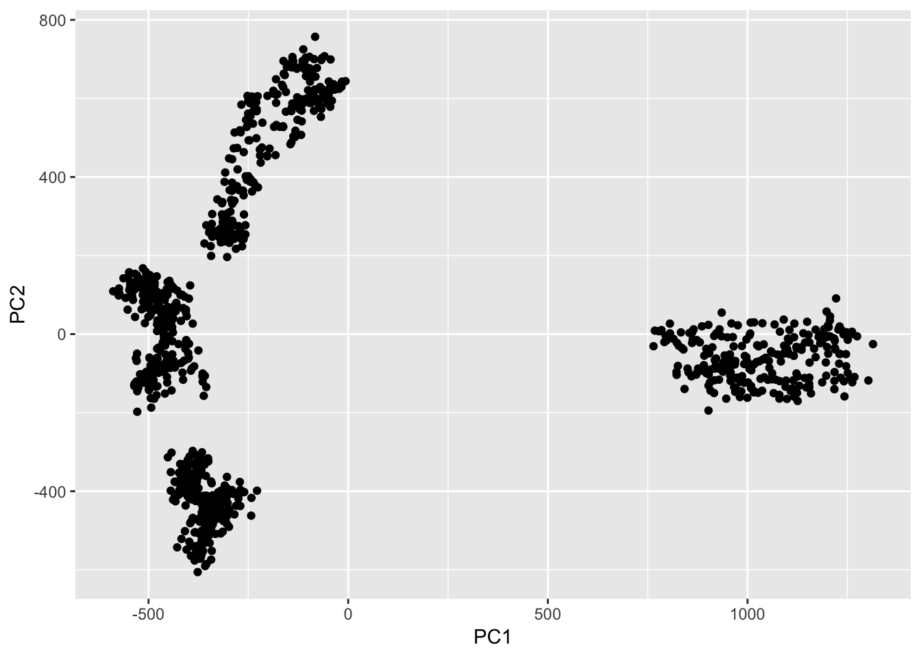
The kMeans function let’s us do k-Means clustering.
set.seed(50)
cluster_pca <- kmeans(pca$x[, 1:10], 4)
cluster_feature <- kmeans(vgg16_feature_list[, -1], 4)
Let’s combine the resulting cluster information back with the image information and create a column class (abbreviated with the first three letters).
cluster_list <- data.frame(cluster_pca = cluster_pca$cluster,
                           cluster_feature = cluster_feature$cluster,
                           vgg16_feature_list) %>%
  select(cluster_pca, cluster_feature, image) %>%
  mutate(class = gsub("/Users/shiringlander/Documents/Github/DL_AI/Tutti_Frutti/fruits-360/Training/", "", image),
         class = substr(class, start = 1, stop = 3))
head(cluster_list)
## cluster_pca cluster_feature
## 1 3 2
## 2 3 2
## 3 3 2
## 4 3 2
## 5 3 2
## 6 3 2
## image
## 1 /Users/shiringlander/Documents/Github/DL_AI/Tutti_Frutti/fruits-360/Training/Cocos/100_100.jpg
## 2 /Users/shiringlander/Documents/Github/DL_AI/Tutti_Frutti/fruits-360/Training/Cocos/101_100.jpg
## 3 /Users/shiringlander/Documents/Github/DL_AI/Tutti_Frutti/fruits-360/Training/Cocos/102_100.jpg
## 4 /Users/shiringlander/Documents/Github/DL_AI/Tutti_Frutti/fruits-360/Training/Cocos/103_100.jpg
## 5 /Users/shiringlander/Documents/Github/DL_AI/Tutti_Frutti/fruits-360/Training/Cocos/104_100.jpg
## 6 /Users/shiringlander/Documents/Github/DL_AI/Tutti_Frutti/fruits-360/Training/Cocos/105_100.jpg
## class
## 1 Coc
## 2 Coc
## 3 Coc
## 4 Coc
## 5 Coc
## 6 CocAnd let’s count the number of images in each cluster, as well their class.
- PCA:
cluster_list %>%
  count(cluster_pca, class)
## # A tibble: 4 x 3
## cluster_pca class n
## <int> <chr> <int>
## 1 1 Sal 245
## 2 2 Coc 245
## 3 3 Coc 245
## 4 4 Sal 245- Original feature map:
cluster_list %>%
  count(cluster_feature, class)
## # A tibble: 4 x 3
## cluster_feature class n
## <int> <chr> <int>
## 1 1 Sal 245
## 2 2 Coc 490
## 3 3 Sal 157
## 4 4 Sal 88The classes map pretty clearly to the four clusters from the PCA.
cluster_list %>%
  mutate(PC1 = pca$x[, 1],
         PC2 = pca$x[, 2]) %>%
  ggplot(aes(x = PC1, y = PC2, color = class, shape = factor(cluster_pca))) +
    geom_point()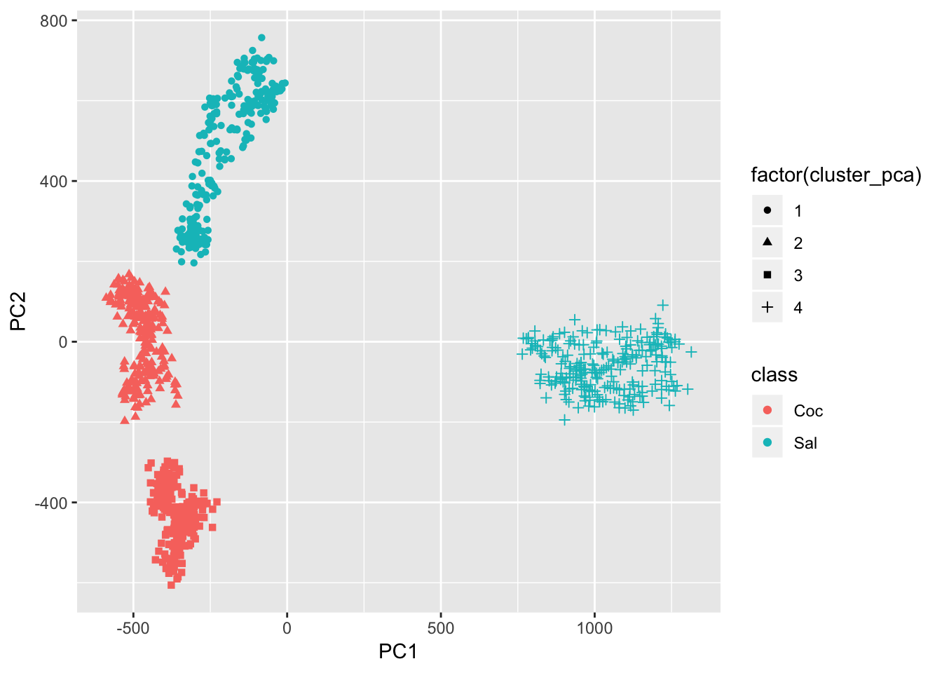
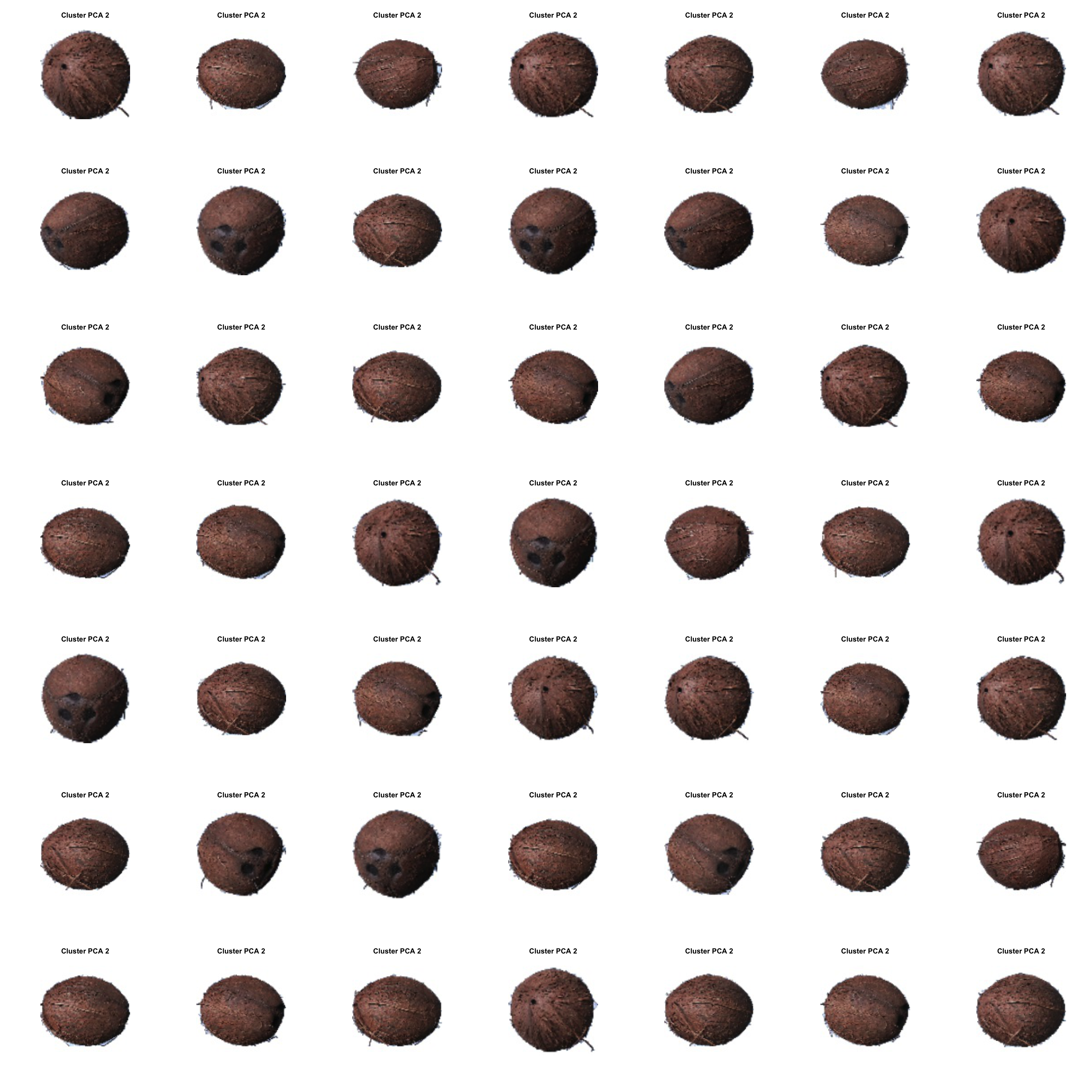
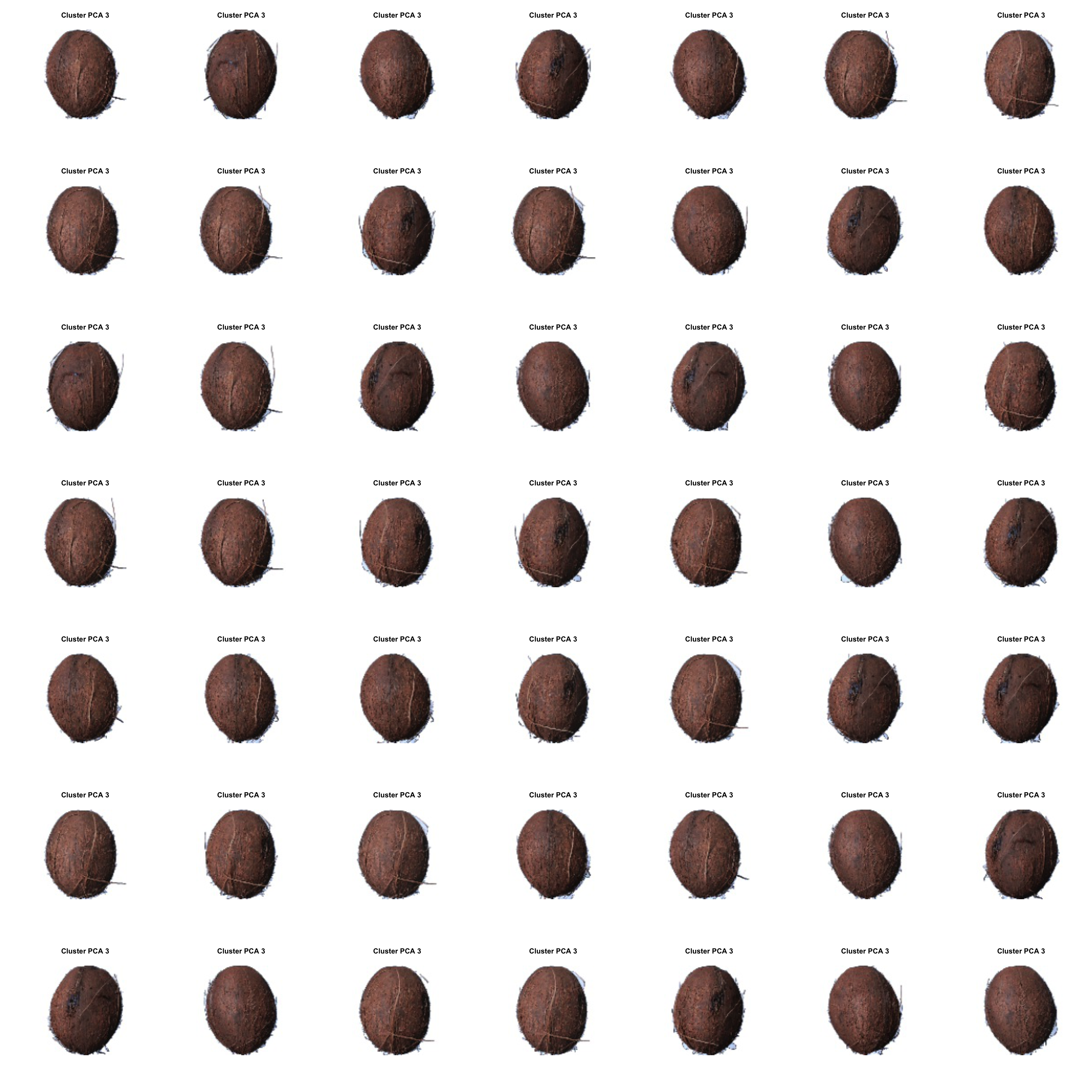
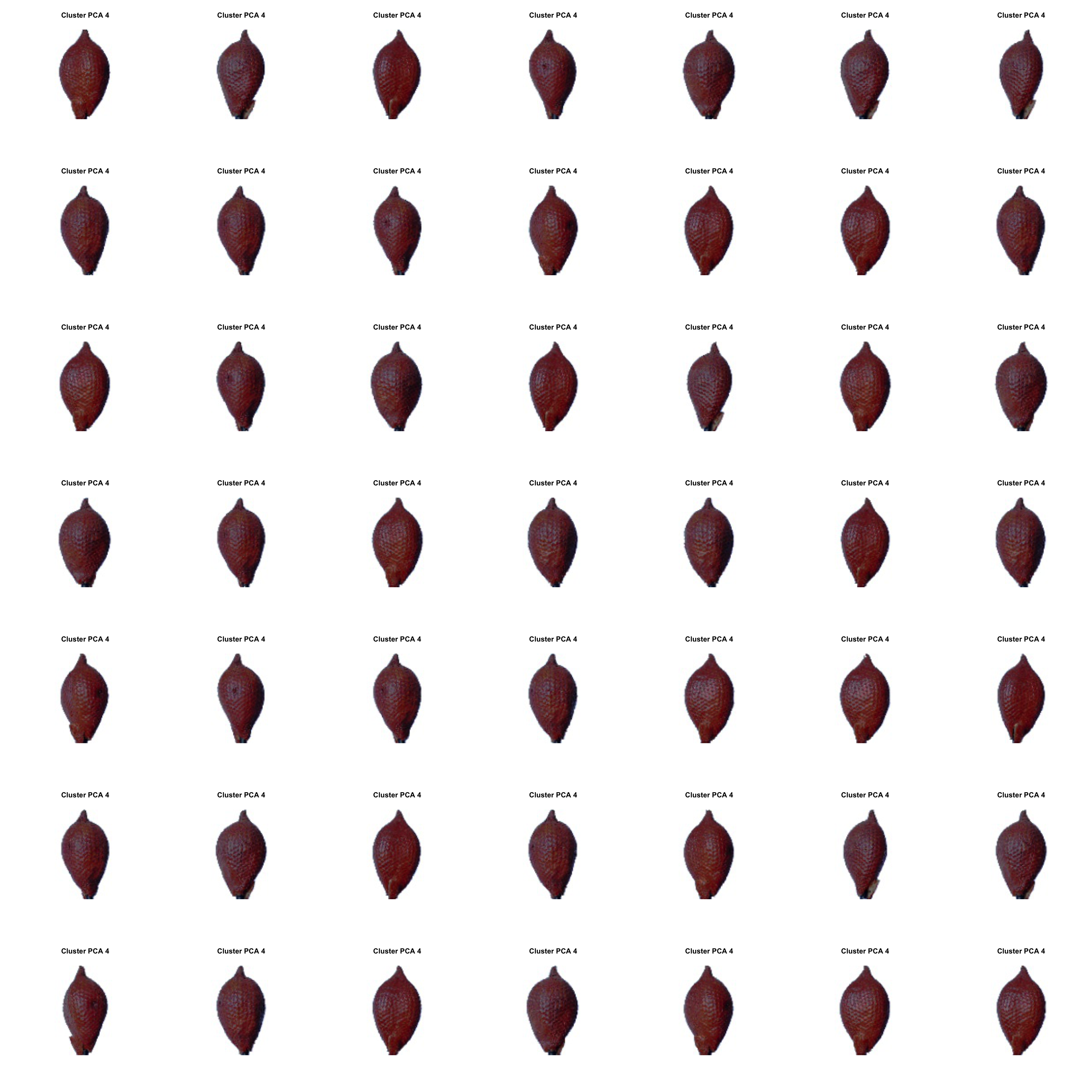
So, let’s plot a few of the images from each cluster so that maybe we’ll be able to see a pattern that explains why our fruits fall into four instead of 2 clusters.
plot_random_images <- function(n_img = 49,
                               cluster = 1,
                               rows = 7,
                               cols = 7) {
  cluster_list_random_cl_1 <- cluster_list %>%
    filter(cluster_pca == cluster) %>%
    sample_n(n_img)

  graphics::layout(matrix(c(1:n_img), rows, cols, byrow = TRUE))
  for (i in 1:n_img) {
    path <- as.character(cluster_list_random_cl_1$image[i])
    img <- load.image(path)
    plot(img, axes = FALSE)
    title(main = paste("Cluster PCA", cluster))
  }
}
sapply(c(1:4), function(x) plot_random_images(cluster = x))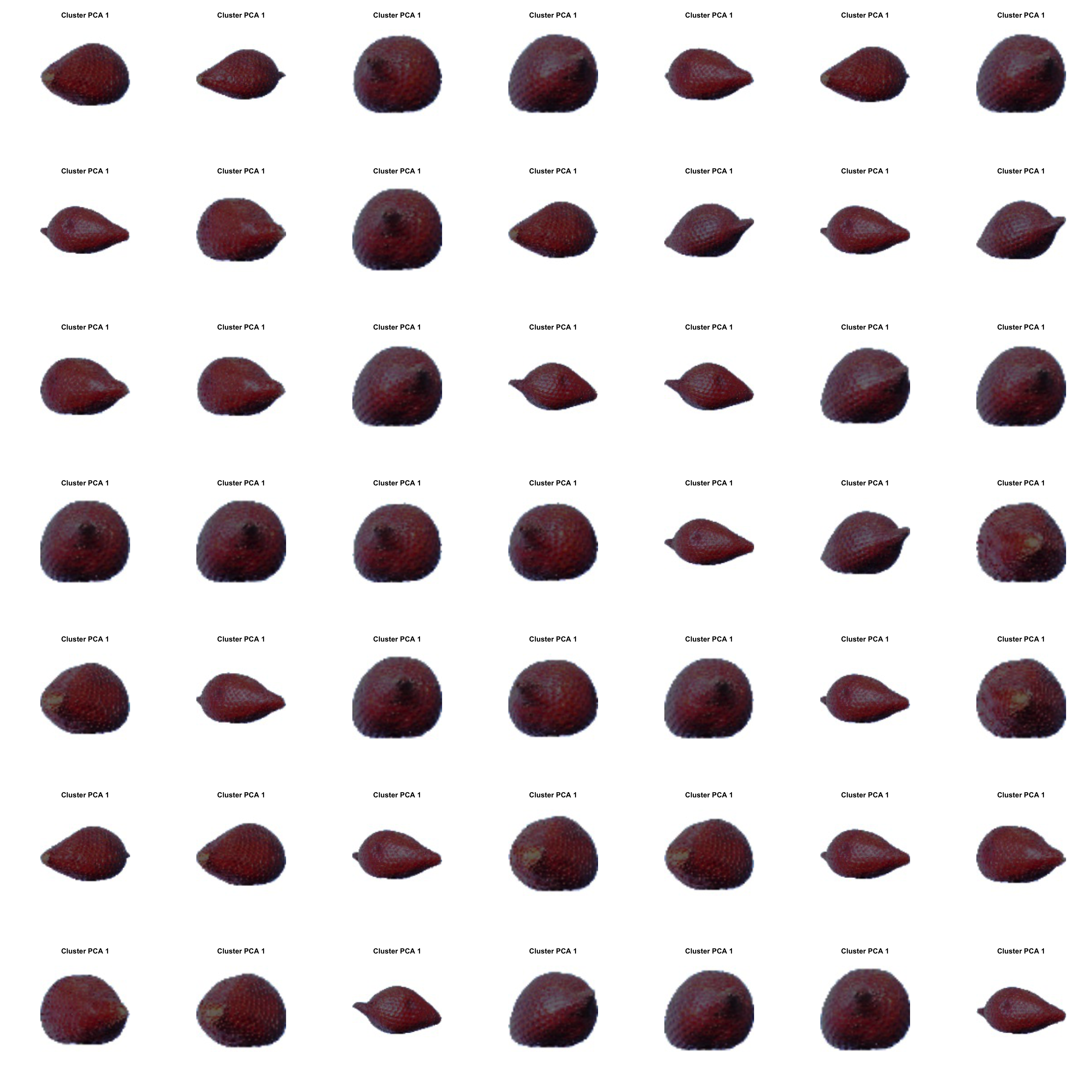
## [[1]]
## NULL
##
## [[2]]
## NULL
##
## [[3]]
## NULL
##
## [[4]]
## NULL
Obviously, the clusters reflect the fruits AND the orientation of the fruits. In that way, our clustering represents intuitive patterns in the images that we can understand.
If we didn’t know the classes, labelling our fruits would be much easier now than manually going through each image individually!
sessionInfo()## R version 3.5.1 (2018-07-02)
## Platform: x86_64-apple-darwin15.6.0 (64-bit)
## Running under: macOS High Sierra 10.13.6
##
## Matrix products: default
## BLAS: /Library/Frameworks/R.framework/Versions/3.5/Resources/lib/libRblas.0.dylib
## LAPACK: /Library/Frameworks/R.framework/Versions/3.5/Resources/lib/libRlapack.dylib
##
## locale:
## [1] de_DE.UTF-8/de_DE.UTF-8/de_DE.UTF-8/C/de_DE.UTF-8/de_DE.UTF-8
##
## attached base packages:
## [1] stats graphics grDevices utils datasets methods base
##
## other attached packages:
## [1] bindrcpp_0.2.2 imager_0.41.1 magrittr_1.5 forcats_0.3.0
## [5] stringr_1.3.1 dplyr_0.7.6 purrr_0.2.5 readr_1.1.1
## [9] tidyr_0.8.1 tibble_1.4.2 ggplot2_3.0.0 tidyverse_1.2.1
## [13] magick_2.0 keras_2.2.0
##
## loaded via a namespace (and not attached):
## [1] Rcpp_0.12.19 lubridate_1.7.4 lattice_0.20-35 png_0.1-7
## [5] utf8_1.1.4 assertthat_0.2.0 zeallot_0.1.0 rprojroot_1.3-2
## [9] digest_0.6.17 tiff_0.1-5 R6_2.3.0 cellranger_1.1.0
## [13] plyr_1.8.4 backports_1.1.2 evaluate_0.11 httr_1.3.1
## [17] blogdown_0.8 pillar_1.3.0 tfruns_1.4 rlang_0.2.2
## [21] lazyeval_0.2.1 readxl_1.1.0 rstudioapi_0.8 whisker_0.3-2
## [25] bmp_0.3 Matrix_1.2-14 reticulate_1.10 rmarkdown_1.10
## [29] labeling_0.3 igraph_1.2.2 munsell_0.5.0 broom_0.5.0
## [33] compiler_3.5.1 modelr_0.1.2 xfun_0.3 pkgconfig_2.0.2
## [37] base64enc_0.1-3 tensorflow_1.9 htmltools_0.3.6 readbitmap_0.1.5
## [41] tidyselect_0.2.4 bookdown_0.7 fansi_0.4.0 crayon_1.3.4
## [45] withr_2.1.2 grid_3.5.1 nlme_3.1-137 jsonlite_1.5
## [49] gtable_0.2.0 scales_1.0.0 cli_1.0.1 stringi_1.2.4
## [53] xml2_1.2.0 tools_3.5.1 glue_1.3.0 hms_0.4.2
## [57] jpeg_0.1-8 yaml_2.2.0 colorspace_1.3-2 rvest_0.3.2
## [61] knitr_1.20 bindr_0.1.1 haven_1.1.2