How to prepare data for NLP (text classification) with Keras and TensorFlow
In the past, I have written and taught quite a bit about image classification with Keras (e.g. here). Text classification isn’t too different in terms of using the Keras principles to train a sequential or function model. You can even use Convolutional Neural Nets (CNNs) for text classification.
What is very different, however, is how to prepare raw text data for modeling. When you look at the IMDB example from the Deep Learning with R Book, you get a great explanation of how to train the model. But because the preprocessed IMDB dataset comes with the keras package, it isn’t so straight-forward to use what you learned on your own data.
How can a computer work with text?
As with any neural network, we need to convert our data into a numeric format; in Keras and TensorFlow we work with tensors. The IMDB example data from the keras package has been preprocessed to a list of integers, where every integer corresponds to a word arranged by descending word frequency.
So, how do we make it from raw text to such a list of integers? Luckily, Keras offers a few convenience functions that make our lives much easier.
library(keras)
library(tidyverse)
Data
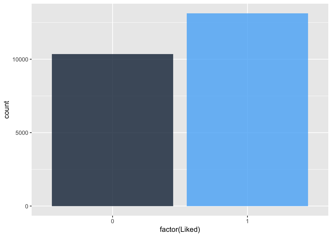
In the example below, I am using a Kaggle dataset: Women’s e-commerce cloting reviews. The data contains a text review of different items of clothing, as well as some additional information, like rating, division, etc. I will use the review title and text in order to classify whether or not the item was liked. I am creating the response variable from the rating: every item rates with 5 stars is considered “liked” (1), the rest as “not liked” (0). I am also combining review title and text.
clothing_reviews <- read_csv("/Users/shiringlander/Documents/Github/ix_lime_etc/Womens Clothing E-Commerce Reviews.csv") %>%
  mutate(Liked = ifelse(Rating == 5, 1, 0),
         text = paste(Title, `Review Text`),
         text = gsub("NA", "", text))
## Parsed with column specification:
## cols(
## X1 = col_double(),
## `Clothing ID` = col_double(),
## Age = col_double(),
## Title = col_character(),
## `Review Text` = col_character(),
## Rating = col_double(),
## `Recommended IND` = col_double(),
## `Positive Feedback Count` = col_double(),
## `Division Name` = col_character(),
## `Department Name` = col_character(),
## `Class Name` = col_character()
## )glimpse(clothing_reviews)## Observations: 23,486
## Variables: 13
## $ X1 <dbl> 0, 1, 2, 3, 4, 5, 6, 7, 8, 9, 10, 11, …
## $ `Clothing ID` <dbl> 767, 1080, 1077, 1049, 847, 1080, 858,…
## $ Age <dbl> 33, 34, 60, 50, 47, 49, 39, 39, 24, 34…
## $ Title <chr> NA, NA, "Some major design flaws", "My…
## $ `Review Text` <chr> "Absolutely wonderful - silky and sexy…
## $ Rating <dbl> 4, 5, 3, 5, 5, 2, 5, 4, 5, 5, 3, 5, 5,…
## $ `Recommended IND` <dbl> 1, 1, 0, 1, 1, 0, 1, 1, 1, 1, 0, 1, 1,…
## $ `Positive Feedback Count` <dbl> 0, 4, 0, 0, 6, 4, 1, 4, 0, 0, 14, 2, 2…
## $ `Division Name` <chr> "Initmates", "General", "General", "Ge…
## $ `Department Name` <chr> "Intimate", "Dresses", "Dresses", "Bot…
## $ `Class Name` <chr> "Intimates", "Dresses", "Dresses", "Pa…
## $ Liked <dbl> 0, 1, 0, 1, 1, 0, 1, 0, 1, 1, 0, 1, 1,…
## $ text <chr> " Absolutely wonderful - silky and sex…Whether an item was liked or not will be the response variable or label for classification of the reviews.
clothing_reviews %>%
  ggplot(aes(x = factor(Liked), fill = Liked)) +
    geom_bar(alpha = 0.8) +
    guides(fill = FALSE)
Tokenizers
The first step is to tokenize the text. This means, converting our text into a sequence of integers where each integer corresponds to a word in the dictionary.
text <- clothing_reviews$textThe num_words argument defines the number of words we want to consider (this will be our feature space). Because the output integers will be sorted according to decreasing word frequency, if we set 1000, we will only get the 1000 most frequent words in our corpus.
max_features <- 1000
tokenizer <- text_tokenizer(num_words = max_features)
Next, we need to fit the tokenizer to our text data. Note, that the tokenizer object is modified in place (as are models in Keras)!
tokenizer %>%
  fit_text_tokenizer(text)
After fitting the tokenizer, we can extract the following information: the number of documents …
tokenizer$document_count## [1] 23486… and the word-index list. Notice, that even though we set the maximum number of words to 1000, our index contains many more words. In fact, the index will keep all words in the index but when converting our reviews to vectors, the stored value tokenizer$num_words will be used to restrict to the most common words.
tokenizer$word_index %>%
  head()
## $raining
## [1] 13788
##
## $yellow
## [1] 553
##
## $four
## [1] 1501
##
## $bottons
## [1] 7837
##
## $woods
## [1] 7896
##
## $`friend's`
## [1] 3525We now have the dictionary of integers and which words they should replace in our text. But we still don’t have a list of integers for our reviews. So, now we use the texts_to_sequences functions, which will do just that! Words, which weren’t among the top 1000 were excluded.
text_seqs <- texts_to_sequences(tokenizer, text)

text_seqs %>%
  head()
## [[1]]
## [1] 249 494 924 3 595 3 63
##
## [[2]]
## [1] 19 7 17 35 84 2 8 221 5 9 4 114 3 37 328 2 135
## [18] 2 421 43 25 57 5 139 35 95 2 75 4 95 3 39 518 2
## [35] 19 1 88 11 31 423 38 4 56 474 1 401 43 160 30 4 132
## [52] 11 447 444 6 761 95
##
## [[3]]
## [1] 156 134 2 68 314 180 12 7 17 3 53 183 5 8 98 12 31
## [18] 2 57 1 95 42 18 240 22 10 2 230 7 8 30 42 15 42
## [35] 9 683 21 2 122 20 803 5 45 2 5 9 95 99 86 16 38
## [52] 581 256 1 24 673 16 63 3 26 267 10 1 182 673 68 4 23
## [69] 148 285 489 3 543 738 481 157 997 4 134 16 1 157 489 846 326
## [86] 1 455 5 706
##
## [[4]]
## [1] 18 292 220 2 19 19 19 7 592 35 209 3 652 310 189 2 33
## [18] 5 2 120 530 10 27 212
##
## [[5]]
## [1] 55 71 7 71 6 23 55 8 76 504 8 1 163 484 5 6 1
## [18] 49 88 8 33 14 262 3 5 6 15 5 855 64 14 257 376 19
## [35] 7 71
##
## [[6]]
## [1] 20 12 1 23 95 2 19 244 10 7 60 6 20 12 1 23 95
## [18] 2 39 38 285 278 324 3 115 33 4 9 7 492 7 17 16 23
## [35] 84 66 13 1 10 250 4 245 13 17 1 100 6 90 3 23 321
## [52] 15 5 18 42 428 20 4 8 3 1 100 43 378 506 111 1 13
## [69] 1 2 19 1 46 3 1 686 13 1 124 10 5 38 135 20 98
## [86] 11 31 2 370 7 17So, there we have it! From here on out, we can simply follow the IMDB example from the Keras documentation:
# Set parameters:
maxlen <- 100
batch_size <- 32
embedding_dims <- 50
filters <- 64
kernel_size <- 3
hidden_dims <- 50
epochs <- 5
Because we can’t directly use this list of integers in our neural network, there is still some preprocessing to do. In the IMDB example, the lists are padded so that they all have the same length. The pad_sequences function will return a matrix, with columns for a given maximum number of words (or the number of words in the longest sequence). Here, we have 400 columns in our matrix. Reviews with fewer words were padded with zeros at the beginning before the indices. Longer reviews are cut after 400 words.
x_train <- text_seqs %>%
  pad_sequences(maxlen = maxlen)
dim(x_train)
## [1] 23486 100Our response variable will be encoded with 1s (5-star review) and 0s (not 5-star reviews). Because we have a binary outcome, we only need this one vector.
y_train <- clothing_reviews$Liked
length(y_train)
## [1] 23486Embeddings
These padded word index matrices now need to be converted into something that gives information about the features (i.e. words) in a way that can be used for learning. Currently, the state-of-the-art for text models are word embeddings or word vectors, which are learned from the text data. Word embeddings encode the context of words in relatively few dimensions while maximizing the information that is contained in these vectors. Basically, word embeddings are values that are learned by a neural net just as weights are learned by a multi-layer perceptron.
Word embedding vectors represent the words and their contexts; thus, words with similar meanings (synonyms) or with close semantic relationships will have more similar embeddings. Moreover, word embeddings should reflect how words are related to each other. For example, the embeddings for “man” should be to “king” as “woman” is to “queen”.
In our model below, we want to learn the word embeddings from our (padded) word vectors and directly use these learned embeddings for classification. This part can now be the same as in the Keras examples for LSTMs and CNNs
model <- keras_model_sequential() %>%
  layer_embedding(max_features, embedding_dims, input_length = maxlen) %>%
  layer_dropout(0.2) %>%
  layer_conv_1d(
    filters, kernel_size,
    padding = "valid", activation = "relu", strides = 1
  ) %>%
  layer_global_max_pooling_1d() %>%
  layer_dense(hidden_dims) %>%
  layer_dropout(0.2) %>%
  layer_activation("relu") %>%
  layer_dense(1) %>%
  layer_activation("sigmoid") %>% compile(
  loss = "binary_crossentropy",
  optimizer = "adam",
  metrics = "accuracy"
)
hist <- model %>%
fit(
x_train,
y_train,
batch_size = batch_size,
epochs = epochs,
validation_split = 0.3
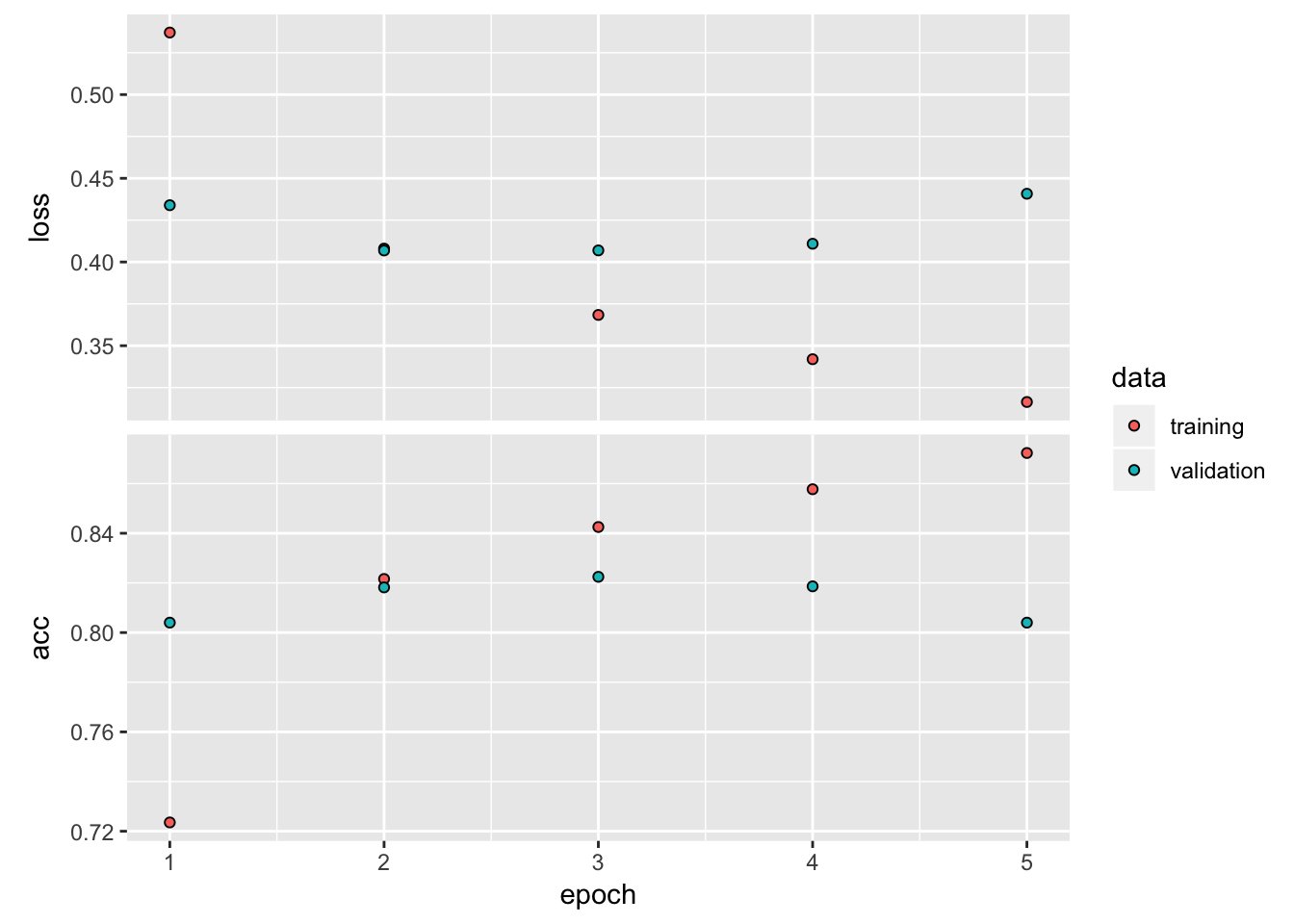
)plot(hist)
Alternative preprocessing functions
The above example follows the IMDB example from the Keras documentation, but there are alternative ways to preprocess your text for modeling with Keras:
one_hot_results <- texts_to_matrix(tokenizer, text, mode = "binary")
dim(one_hot_results)
## [1] 23486 1000hashing_results <- text_hashing_trick(text[1], n = 100)
hashing_results## [1] 88 75 18 90 7 90 23Pretrained embeddings
Here, we have learned word embeddings from our word vectors and directly used the output of the embedding layers as input for additional layers in our neural net. Because learning embeddings takes time and computational power, we could also start with pre-trained embeddings, particulary if we don’t have a whole lot of training data. You can find an example for how to use GloVe embeddings here.
Session info
sessionInfo()## R version 3.5.2 (2018-12-20)
## Platform: x86_64-apple-darwin15.6.0 (64-bit)
## Running under: macOS Mojave 10.14.2
##
## Matrix products: default
## BLAS: /Library/Frameworks/R.framework/Versions/3.5/Resources/lib/libRblas.0.dylib
## LAPACK: /Library/Frameworks/R.framework/Versions/3.5/Resources/lib/libRlapack.dylib
##
## locale:
## [1] en_US.UTF-8/en_US.UTF-8/en_US.UTF-8/C/en_US.UTF-8/en_US.UTF-8
##
## attached base packages:
## [1] stats graphics grDevices utils datasets methods base
##
## other attached packages:
## [1] bindrcpp_0.2.2 forcats_0.3.0 stringr_1.3.1 dplyr_0.7.8
## [5] purrr_0.2.5 readr_1.3.1 tidyr_0.8.2 tibble_2.0.1
## [9] ggplot2_3.1.0 tidyverse_1.2.1 keras_2.2.4
##
## loaded via a namespace (and not attached):
## [1] reticulate_1.10 tidyselect_0.2.5 xfun_0.4 reshape2_1.4.3
## [5] haven_2.0.0 lattice_0.20-38 colorspace_1.4-0 generics_0.0.2
## [9] htmltools_0.3.6 yaml_2.2.0 base64enc_0.1-3 utf8_1.1.4
## [13] rlang_0.3.1 pillar_1.3.1 withr_2.1.2 glue_1.3.0
## [17] readxl_1.2.0 modelr_0.1.2 bindr_0.1.1 plyr_1.8.4
## [21] tensorflow_1.10 cellranger_1.1.0 munsell_0.5.0 blogdown_0.10
## [25] gtable_0.2.0 rvest_0.3.2 evaluate_0.12 labeling_0.3
## [29] knitr_1.21 tfruns_1.4 fansi_0.4.0 broom_0.5.1
## [33] Rcpp_1.0.0 backports_1.1.3 scales_1.0.0 jsonlite_1.6
## [37] hms_0.4.2 digest_0.6.18 stringi_1.2.4 bookdown_0.9
## [41] grid_3.5.2 cli_1.0.1 tools_3.5.2 magrittr_1.5
## [45] lazyeval_0.2.1 crayon_1.3.4 whisker_0.3-2 pkgconfig_2.0.2
## [49] zeallot_0.1.0 Matrix_1.2-15 xml2_1.2.0 lubridate_1.7.4
## [53] rstudioapi_0.9.0 assertthat_0.2.0 rmarkdown_1.11 httr_1.4.0
## [57] R6_2.3.0 nlme_3.1-137 compiler_3.5.2