Baby Weight Shiny app
Alright, this is it: I am officially back! :-D
I have not written any blogposts for over a year. Last year, I had the cutest baby boy and ever since then, I did not get around to doing much coding. One of the reasons was that, unfortunately, we did not have the easiest of starts with the little one. Feeding problems led to weight gain problems, so we had to weigh him regularly. Because I wanted to see for myself if we were on the right track with his weight gain, I created this Baby Weight Shiny app. With the app, I could easily visualize how we compared to the WHO baby/childen weight-for-age tables.
Below, I’ll describe how I prepared the data and built the plots. The entire code for building the app can be found on Github.
If you have questions or would like to talk about the app (or something else data-related), you can now book 15-minute timeslots with me (it’s free - one slot available per weekday):

If you have been enjoying my content and would like to help me be able to create more, please consider sending me a donation at . Thank you! :-)
Reference data
I am using the following WHO baby/childen weight-for-age tables:
- Percentiles girls & boys
I combined girls’ and boys’ data into one table each for:
- Weight-for-age: Birth to 13 weeks
- Weight-for-age: Birth to 5 years
Adding my own measurements
I collected all our weight measurements in a .csv file with two columns:
- a
datecolumn in the format%d.%m.%Y(dd.mm.yyyy) - a
weightcolumn in g or kg
The first row has to contain the birthdate and birthweight, as this is what’s used to calculate the growth percentile to follow. A baby’s birthweight will put them into a certain growth percentile (e.g. a boy who weighs around 3.3 kg at birth is closest to the 50th percentile, meaning that about 50% of boys his same age will be heavier and 50% will be lighter than he is). For a healthy weight gain, the baby’s weight curve is supposed to roughly follow a parallel line with this growth percentile.
Because, obviously, I am not going to make my son’s actual weight data available on the internet, I created some mock data, similar to real-world examples (weight in g):
library(readr)
library(lubridate)

# download from https://github.com/ShirinG/who_baby_weight_app/
weight_measures <- read_delim("weight_measures.csv",
                            delim = ",",
                            col_types = list(col_date(format = "%d.%m.%Y"), col_double()))
head(weight_measures)
## # A tibble: 6 x 2
## date weight
## <date> <dbl>
## 1 2019-08-12 3168
## 2 2019-08-16 3126
## 3 2019-08-17 3138
## 4 2019-08-18 3348
## 5 2019-08-20 3286
## 6 2019-08-22 3626In the Baby Weight Shiny app, you can upload this mock data or your own data. Then choose:
- whether the columns in your
.csvare separated by comma, semicolon or tabulator - whether you want to show only reference values for the first 13 weeks or for the first 5 years (only reference values corresponding to your measurement dates will be shown)
- whether your weight data is given in gramm or kilogramm and
- whether you want to display reference data for girls or boys
You can then check to see if the data looks correct (tab: Data). The tabs Curve and Barchart show two plots. Below, I’ll describe how I prepared the data for plotting.
Data preparation
First, I combined my weight measures with the reference tables from WHO. The function is saved in a script on Github for you to examine. The function code contains comments that describe what I’ve been doing. Here is the outcome:
library(tidyverse)

# download from https://github.com/ShirinG/who_baby_weight_app/
source("combine_measures.R")
p_0_5 <- read_csv("p_0_5.csv")
p_0_13 <- read_csv("p_0_13.csv")

combine_measures_who_final <- combine_measures_who(weight_measures,
                                                   p_0_13, p_0_5,
                                                   age_range = "0_5",
                                                   weight_in = "g",
                                                   gender = "boy")
head(combine_measures_who_final)
## # A tibble: 6 x 10
## date weight ref percentile starting_p Month L M S gender
## <date> <dbl> <chr> <chr> <chr> <dbl> <dbl> <dbl> <dbl> <chr>
## 1 2019-08-12 3.17 measur… measureme… P50 NA NA NA NA <NA>
## 2 2019-08-16 3.13 measur… measureme… P50 NA NA NA NA <NA>
## 3 2019-08-17 3.14 measur… measureme… P50 NA NA NA NA <NA>
## 4 2019-08-18 3.35 measur… measureme… P50 NA NA NA NA <NA>
## 5 2019-08-20 3.29 measur… measureme… P50 NA NA NA NA <NA>
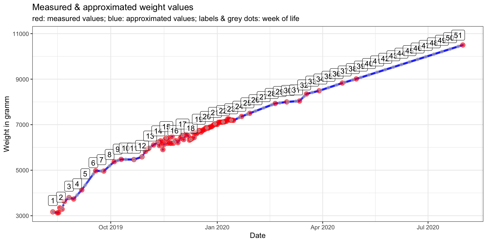
## 6 2019-08-22 3.63 measur… measureme… P50 NA NA NA NA <NA>In order to calculate weight data for every full week of life (to make the values comparable with the reference), I am interpolating weight values for every day with missing information (linear approximation).
# add missing dates for calculating weight change per week of life
reference_date <- weight_measures$date[[1]]
end_date <- weight_measures$date[[nrow(weight_measures)]]

starting_p <- combine_measures_who_final %>%
  filter(date == reference_date) %>%
  select(starting_p) %>%
  .[[1]] %>%
  .[1]

all_dates <- seq(from = reference_date, to = end_date, by = "day") %>%
  as_tibble()
colnames(all_dates) = "date"

weight_measures_all <- weight_measures %>%
  full_join(all_dates, by = "date") %>%
  arrange(date)

## approximate missing values
weight_measures_all <- weight_measures_all %>%
  mutate(weight_approx = approx(weight, n = nrow(.))[[2]])

## add running week number
nos <- rep(1:ceiling(nrow(weight_measures_all)/7), each = 7)
weight_measures_all$week <- nos[1:nrow(weight_measures_all)]

## calculate sum over week
weight_measures_all <- weight_measures_all %>%
  mutate(diff_day = c(0, diff(weight_approx, lag = 1)),
         diff_week = c(rep(0, 7), diff(weight_approx, lag = 7)))
I also want to know the month of life, so I am using the following function to do so:
# download from https://github.com/ShirinG/who_baby_weight_app/
source("elapsed_months.R")
weight_measures_all <- weight_measures_all %>%
  mutate(month = elapsed_months(date, reference_date))
The curve
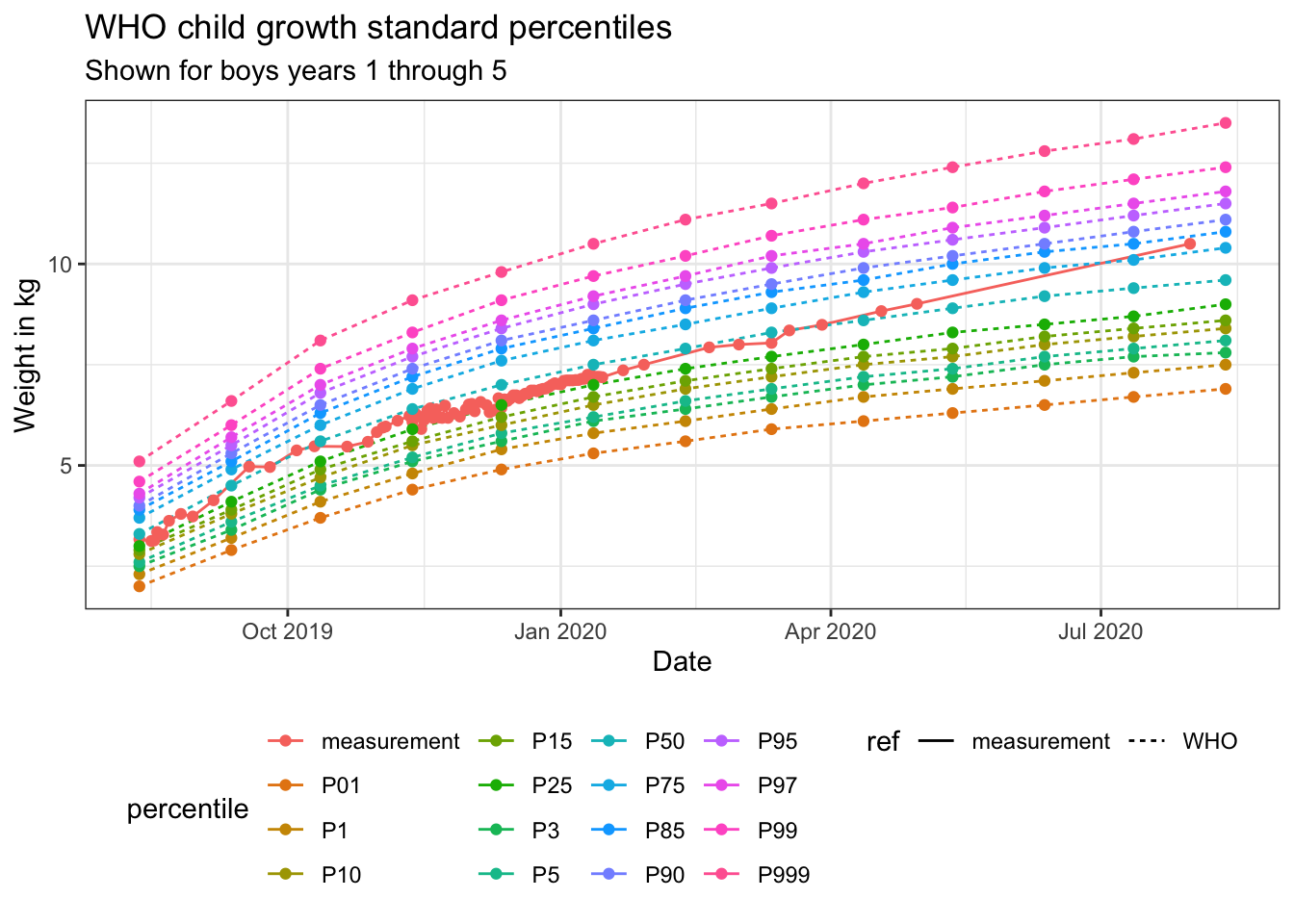
The first plot shows a simple lineplot with all reference curves (i.e. all WHO growth percentiles) and my measurements plotted against them. The plot in the Shiny app has been created with Plotly, so you can click on the legend to hide/show specific growth percentiles or zoom into specific areas on the plot.
gender <- "boys"
age <- "years 1 through 5"

combine_measures_who_final %>%
  ggplot(aes(date, weight,
             linetype = ref,
             color = percentile)) +
    geom_line() +
    geom_point() +
    labs(x = "Date",
         y = "Weight in kg",
         title = "WHO child growth standard percentiles",
         subtitle = paste("Shown for", gender, age)) +
    theme_bw() +
    theme(legend.position = "bottom")
test_curves <- combine_measures_who_final %>%
  filter(percentile == !!paste(starting_p)) %>%
  left_join(select(weight_measures_all, date, weight_approx), by = "date")

paste("Your reference percentile is:", starting_p)
## [1] "Your reference percentile is: P50"paste("Correlation between your measurements and your reference percentile is:",
round(cor(test_curves$weight, test_curves$weight_approx, use = 'complete.obs'), digits = 5))## [1] "Correlation between your measurements and your reference percentile is: 0.98757"Approximated missing values
The next plot is not shown in the Shiny app, but here I’ll include it to show how the interpolated weight values look like:
weight_measures_all %>%
  ggplot(aes(x = date)) +
    geom_line(aes(y = weight_approx), color = "grey") +
    geom_point(aes(y = weight_approx), color = "blue", size = 1, alpha = 0.6) +
    geom_point(aes(y = weight), color = "red", size = 3, alpha = 0.6) +
    geom_point(data = weight_measures_all %>% distinct(week, .keep_all = TRUE),
               aes(x = date, y = weight_approx),
               color = "grey", size = 2, alpha = 0.6) +
    geom_label(data = weight_measures_all %>% distinct(week, .keep_all = TRUE),
               aes(x = date, y = weight_approx, label = week),
               nudge_y = 500, alpha = 0.6) +
    labs(x = "Date",
         y = "Weight in gramm",
         title = "Measured & approximated weight values",
         subtitle = "red: measured values; blue: approximated values; labels & grey dots: week of life") +
    theme_bw()
Barchart
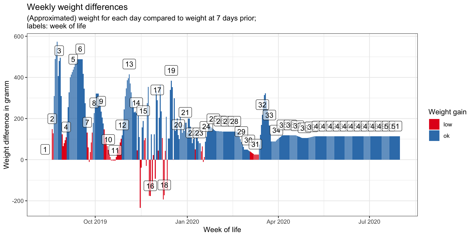
The barchart, which you can find in the Shiny app, shows weekly weight differences, i.e. for every day the difference in weight compared to 7 days prior is calculated.
Bar colors show whether the weekly weight difference is above (blue) or below (red) the required minimum for BREASTFED babies given by this German site about breastfeeding:
- in months 1 and 2, the minimum weight gain should be: 170 g
- in months 3 and 4: 110 g
- in months 5 and 6: 70 g and
- from month 7 to 12: 40 g
Update: Based on a Github pull request by latlio, I changed the ifelse statement to case_when (thanks again for the contribution!).
weight_measures_all <- weight_measures_all %>%
            mutate(color = case_when(
                month <= 2 & diff_week >= 170 ~ "ok",
                month == 3 & diff_week >= 110 ~ "ok",
                month == 4 & diff_week >= 110 ~ "ok",
                month == 5 & diff_week >= 70 ~ "ok",
                month == 6 & diff_week >= 70 ~ "ok",
                month >= 7 & diff_week >= 40 ~ "ok",
                TRUE ~ "low"))
The actual plot in the Shiny app is again created with Plotly, so you can interact with the graph there.
weight_measures_all %>%
  ggplot(aes(x = date, y = diff_week)) +
    geom_bar(aes(fill = color), stat = "identity") +
    geom_label(data = weight_measures_all %>% distinct(week, .keep_all = TRUE),
               aes(x = date, label = week),
               nudge_y = 50, alpha = 0.6) +
    scale_fill_brewer(palette = "Set1") +
    labs(x = "Week of life",
         y = "Weight difference in gramm",
         fill = "Weight gain",
         title = "Weekly weight differences",
         subtitle = "(Approximated) weight for each day compared to weight at 7 days prior;\nlabels: week of life") +
    theme_bw()
sessionInfo()## R version 4.0.2 (2020-06-22)
## Platform: x86_64-apple-darwin17.0 (64-bit)
## Running under: macOS Catalina 10.15.6
##
## Matrix products: default
## BLAS: /Library/Frameworks/R.framework/Versions/4.0/Resources/lib/libRblas.dylib
## LAPACK: /Library/Frameworks/R.framework/Versions/4.0/Resources/lib/libRlapack.dylib
##
## locale:
## [1] en_US.UTF-8/en_US.UTF-8/en_US.UTF-8/C/en_US.UTF-8/en_US.UTF-8
##
## attached base packages:
## [1] stats graphics grDevices utils datasets methods base
##
## other attached packages:
## [1] forcats_0.5.0 stringr_1.4.0 dplyr_1.0.2 purrr_0.3.4
## [5] tidyr_1.1.2 tibble_3.0.3 ggplot2_3.3.2 tidyverse_1.3.0
## [9] lubridate_1.7.9 readr_1.3.1
##
## loaded via a namespace (and not attached):
## [1] tidyselect_1.1.0 xfun_0.17 haven_2.3.1 colorspace_1.4-1
## [5] vctrs_0.3.4 generics_0.0.2 htmltools_0.5.0 yaml_2.2.1
## [9] utf8_1.1.4 blob_1.2.1 rlang_0.4.7 pillar_1.4.6
## [13] withr_2.2.0 glue_1.4.2 DBI_1.1.0 RColorBrewer_1.1-2
## [17] dbplyr_1.4.4 modelr_0.1.8 readxl_1.3.1 lifecycle_0.2.0
## [21] munsell_0.5.0 blogdown_0.20.1 gtable_0.3.0 cellranger_1.1.0
## [25] rvest_0.3.6 evaluate_0.14 labeling_0.3 knitr_1.29
## [29] fansi_0.4.1 broom_0.7.0 Rcpp_1.0.5 backports_1.1.9
## [33] scales_1.1.1 jsonlite_1.7.1 farver_2.0.3 fs_1.5.0
## [37] hms_0.5.3 digest_0.6.25 stringi_1.5.3 bookdown_0.20
## [41] grid_4.0.2 cli_2.0.2 tools_4.0.2 magrittr_1.5
## [45] crayon_1.3.4 pkgconfig_2.0.3 ellipsis_0.3.1 xml2_1.3.2
## [49] reprex_0.3.0 rstudioapi_0.11 assertthat_0.2.1 rmarkdown_2.3
## [53] httr_1.4.2 R6_2.4.1 compiler_4.0.2