
How to combine point and boxplots in timeline charts with ggplot2 facets
In a recent project, I was looking to plot data from different variables along the same time axis. The difficulty was, that some of these variables I wanted to have as point plots, while others I wanted as box-plots.
Because I work with the tidyverse, I wanted to produce these plots with ggplot2. Faceting was the obvious first step but it took me quite a while to figure out how to best combine facets with point plots (where I have one value per time point) with and box-plots (where I have multiple values per time point).
The reason why this isn’t trivial is that box plots require groups or factors on the x-axis, while points can be plotted over a continuous range of x-values. If your alarm bells are ringing right now, you are absolutely right: before you try to combine plots with different x-axis properties, you should think long and hard whether this is an accurate representation of the data and if its a good idea to do so! Here, I had multiple values per time point for one variable and I wanted to make the median + variation explicitly clear, while also showing the continuous changes of other variables over the same range of time.
So, I am writing this short tutorial here in hopes that it saves the next person trying to do something similar from spending an entire morning on stackoverflow. ;-)
For this demonstration, I am creating some fake data:
library(tidyverse)
dates <- seq(as.POSIXct("2017-10-01 07:00"), as.POSIXct("2017-10-01 10:30"), by = 180) # 180 seconds == 3 minutes
fake_data <- data.frame(time = dates,
                        var1_1 = runif(length(dates)),
                        var1_2 = runif(length(dates)),
                        var1_3 = runif(length(dates)),
                        var2 = runif(length(dates))) %>%
  sample_frac(size = 0.33)
head(fake_data)
## time var1_1 var1_2 var1_3 var2
## 1 2017-10-01 08:33:00 0.4208415 0.2589455 0.3786275 0.80532017
## 2 2017-10-01 08:42:00 0.4853185 0.4949028 0.9104159 0.25552958
## 3 2017-10-01 09:42:00 0.4144495 0.6314172 0.5832432 0.74209701
## 4 2017-10-01 09:54:00 0.9315311 0.8266359 0.1509052 0.55146543
## 5 2017-10-01 08:36:00 0.1212433 0.3228635 0.5638170 0.43761903
## 6 2017-10-01 09:21:00 0.2826186 0.8656590 0.8774104 0.07265883Here, variable 1 (var1) has three measurements per time point, while variable 2 (var2) has one.
First, for plotting with ggplot2 we want our data in a tidy long format. I also add another column for faceting that groups the variables from var1 together.
fake_data_long <- fake_data %>%
  gather(x, y, var1_1:var2) %>%
  mutate(facet = ifelse(x %in% c("var1_1", "var1_2", "var1_3"), "var1", x))
head(fake_data_long)
## time x y facet
## 1 2017-10-01 08:33:00 var1_1 0.4208415 var1
## 2 2017-10-01 08:42:00 var1_1 0.4853185 var1
## 3 2017-10-01 09:42:00 var1_1 0.4144495 var1
## 4 2017-10-01 09:54:00 var1_1 0.9315311 var1
## 5 2017-10-01 08:36:00 var1_1 0.1212433 var1
## 6 2017-10-01 09:21:00 var1_1 0.2826186 var1Now, we can plot this the following way:
- facet by variable
- subset data to facets for point plots and give aesthetics in
geom_point() - subset data to facets for box plots and give aesthetics in
geom_boxplot(). Here we also need to set thegroupaesthetic; if we don’t specifically give that, we will get a plot with one big box, instead of a box for every time point.
fake_data_long %>%
  ggplot() +
    facet_grid(facet ~ ., scales = "free") +
    geom_point(data = subset(fake_data_long, facet == "var2"),
               aes(x = time, y = y),
               size = 1) +
    geom_line(data = subset(fake_data_long, facet == "var2"),
               aes(x = time, y = y)) +
    geom_boxplot(data = subset(fake_data_long, facet == "var1"),
               aes(x = time, y = y, group = time))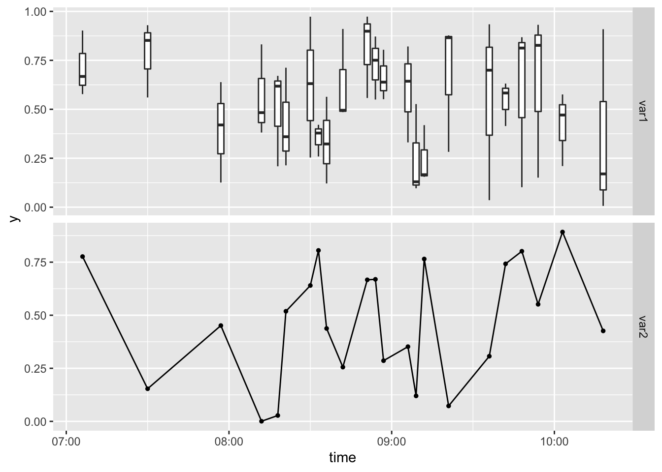
sessionInfo()## R version 4.0.2 (2020-06-22)
## Platform: x86_64-apple-darwin17.0 (64-bit)
## Running under: macOS Catalina 10.15.6
##
## Matrix products: default
## BLAS: /Library/Frameworks/R.framework/Versions/4.0/Resources/lib/libRblas.dylib
## LAPACK: /Library/Frameworks/R.framework/Versions/4.0/Resources/lib/libRlapack.dylib
##
## locale:
## [1] en_US.UTF-8/en_US.UTF-8/en_US.UTF-8/C/en_US.UTF-8/en_US.UTF-8
##
## attached base packages:
## [1] stats graphics grDevices utils datasets methods base
##
## other attached packages:
## [1] forcats_0.5.0 stringr_1.4.0 dplyr_1.0.2 purrr_0.3.4
## [5] readr_1.3.1 tidyr_1.1.2 tibble_3.0.3 ggplot2_3.3.2
## [9] tidyverse_1.3.0
##
## loaded via a namespace (and not attached):
## [1] tidyselect_1.1.0 xfun_0.17 haven_2.3.1 colorspace_1.4-1
## [5] vctrs_0.3.4 generics_0.0.2 htmltools_0.5.0 yaml_2.2.1
## [9] blob_1.2.1 rlang_0.4.7 pillar_1.4.6 glue_1.4.2
## [13] withr_2.2.0 DBI_1.1.0 dbplyr_1.4.4 modelr_0.1.8
## [17] readxl_1.3.1 lifecycle_0.2.0 munsell_0.5.0 blogdown_0.20.1
## [21] gtable_0.3.0 cellranger_1.1.0 rvest_0.3.6 evaluate_0.14
## [25] labeling_0.3 knitr_1.29 fansi_0.4.1 broom_0.7.0
## [29] Rcpp_1.0.5 scales_1.1.1 backports_1.1.10 jsonlite_1.7.1
## [33] farver_2.0.3 fs_1.5.0 hms_0.5.3 digest_0.6.25
## [37] stringi_1.5.3 bookdown_0.20 grid_4.0.2 cli_2.0.2
## [41] tools_4.0.2 magrittr_1.5 crayon_1.3.4 pkgconfig_2.0.3
## [45] ellipsis_0.3.1 xml2_1.3.2 reprex_0.3.0 lubridate_1.7.9
## [49] assertthat_0.2.1 rmarkdown_2.3 httr_1.4.2 rstudioapi_0.11
## [53] R6_2.4.1 compiler_4.0.2