
Explaining Black-Box Machine Learning Models - Code Part 1: tabular data + caret + iml
This is code that will encompany an article that will appear in a special edition of a German IT magazine. The article is about explaining black-box machine learning models. In that article I’m showcasing three practical examples:
- Explaining supervised classification models built on tabular data using
caretand theimlpackage - Explaining image classification models with
kerasandlime - Explaining text classification models with
xgboostandlime
Below, you will find the code for the first part:
# data wrangling
library(tidyverse)
library(readr)

# ml
library(caret)

# plotting
library(gridExtra)
library(grid)
library(ggridges)
library(ggthemes)
theme_set(theme_minimal())

# explaining models
# https://github.com/christophM/iml
library(iml)

# https://pbiecek.github.io/breakDown/
library(breakDown)

# https://pbiecek.github.io/DALEX/
library(DALEX)
Supervised classfication models with tabular data
The data
The example dataset I am using in this part is the wine quality data. Let’s read it in and do some minor housekeeping, like
- converting the response variable
qualityinto two categories with roughly equal sizes and - replacing the spaces in the column names with “_" to make it easier to handle in the tidyverse
wine_data <- read_csv("/Users/shiringlander/Documents/Github/ix_lime_etc/winequality-red.csv") %>%
  mutate(quality = as.factor(ifelse(quality < 6, "qual_low", "qual_high")))
## Parsed with column specification:
## cols(
## `fixed acidity` = col_double(),
## `volatile acidity` = col_double(),
## `citric acid` = col_double(),
## `residual sugar` = col_double(),
## chlorides = col_double(),
## `free sulfur dioxide` = col_double(),
## `total sulfur dioxide` = col_double(),
## density = col_double(),
## pH = col_double(),
## sulphates = col_double(),
## alcohol = col_double(),
## quality = col_integer()
## )colnames(wine_data) <- gsub(" ", "_", colnames(wine_data))
glimpse(wine_data)## Observations: 1,599
## Variables: 12
## $ fixed_acidity <dbl> 7.4, 7.8, 7.8, 11.2, 7.4, 7.4, 7.9, 7.3, ...
## $ volatile_acidity <dbl> 0.700, 0.880, 0.760, 0.280, 0.700, 0.660,...
## $ citric_acid <dbl> 0.00, 0.00, 0.04, 0.56, 0.00, 0.00, 0.06,...
## $ residual_sugar <dbl> 1.9, 2.6, 2.3, 1.9, 1.9, 1.8, 1.6, 1.2, 2...
## $ chlorides <dbl> 0.076, 0.098, 0.092, 0.075, 0.076, 0.075,...
## $ free_sulfur_dioxide <dbl> 11, 25, 15, 17, 11, 13, 15, 15, 9, 17, 15...
## $ total_sulfur_dioxide <dbl> 34, 67, 54, 60, 34, 40, 59, 21, 18, 102, ...
## $ density <dbl> 0.9978, 0.9968, 0.9970, 0.9980, 0.9978, 0...
## $ pH <dbl> 3.51, 3.20, 3.26, 3.16, 3.51, 3.51, 3.30,...
## $ sulphates <dbl> 0.56, 0.68, 0.65, 0.58, 0.56, 0.56, 0.46,...
## $ alcohol <dbl> 9.4, 9.8, 9.8, 9.8, 9.4, 9.4, 9.4, 10.0, ...
## $ quality <fct> qual_low, qual_low, qual_low, qual_high, ...EDA
The first step in my machine learning workflows in exploratory data analysis (EDA). This can get pretty extensive, but here I am only looking at the distributions of my features and the class counts of my response variable.
p1 <- wine_data %>%
  ggplot(aes(x = quality, fill = quality)) +
    geom_bar(alpha = 0.8) +
    scale_fill_tableau() +
    guides(fill = FALSE)
p2 <- wine_data %>%
gather(x, y, fixed_acidity:alcohol) %>%
ggplot(aes(x = y, y = quality, color = quality, fill = quality)) +
facet_wrap( ~ x, scale = "free", ncol = 3) +
scale_fill_tableau() +
scale_color_tableau() +
geom_density_ridges(alpha = 0.8) +
guides(fill = FALSE, color = FALSE)grid.arrange(p1, p2, ncol = 2, widths = c(0.3, 0.7))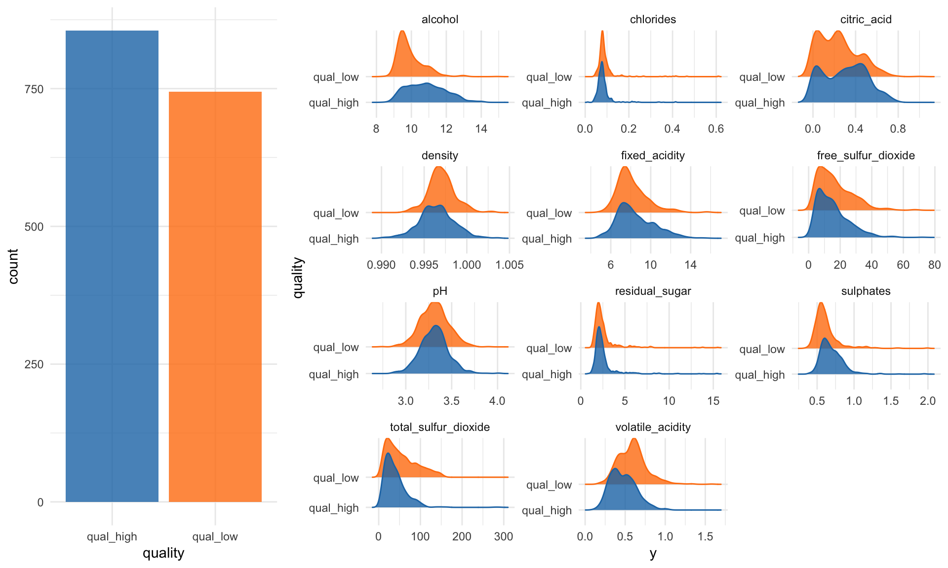
Model
For modeling, I am splitting the data into 80% for training and 20% for testing.
set.seed(42)
idx <- createDataPartition(wine_data$quality,
                           p = 0.8,
                           list = FALSE,
                           times = 1)

wine_train <- wine_data[ idx,]
wine_test  <- wine_data[-idx,]
I am using 5-fold cross-validation, repeated 3x and scale and center the data. The example model I am using here is a Random Forest model.
fit_control <- trainControl(method = "repeatedcv",
                           number = 5,
                           repeats = 3)

set.seed(42)
rf_model <- train(quality ~ .,
                  data = wine_train,
                  method = "rf",
                  preProcess = c("scale", "center"),
                  trControl = fit_control,
verbose = FALSE)rf_model## Random Forest
##
## 1280 samples
## 11 predictor
## 2 classes: 'qual_high', 'qual_low'
##
## Pre-processing: scaled (11), centered (11)
## Resampling: Cross-Validated (5 fold, repeated 3 times)
## Summary of sample sizes: 1023, 1024, 1025, 1024, 1024, 1024, ...
## Resampling results across tuning parameters:
##
## mtry Accuracy Kappa
## 2 0.7958240 0.5898607
## 6 0.7893104 0.5766700
## 11 0.7882738 0.5745067
##
## Accuracy was used to select the optimal model using the largest value.
## The final value used for the model was mtry = 2.Now let’s see how good our model is:
test_predict <- predict(rf_model, wine_test)
confusionMatrix(test_predict, as.factor(wine_test$quality))
## Confusion Matrix and Statistics
##
## Reference
## Prediction qual_high qual_low
## qual_high 140 26
## qual_low 31 122
##
## Accuracy : 0.8213
## 95% CI : (0.7748, 0.8618)
## No Information Rate : 0.5361
## P-Value [Acc > NIR] : <2e-16
##
## Kappa : 0.6416
## Mcnemar's Test P-Value : 0.5962
##
## Sensitivity : 0.8187
## Specificity : 0.8243
## Pos Pred Value : 0.8434
## Neg Pred Value : 0.7974
## Prevalence : 0.5361
## Detection Rate : 0.4389
## Detection Prevalence : 0.5204
## Balanced Accuracy : 0.8215
##
## 'Positive' Class : qual_high
## Okay, this model isn’t too accurate but since my focus here is supposed to be on explaining the model, that’s good enough for me at this point.
Explaining/interpreting the model
There are several methods and tools that can be used to explain or interpret machine learning models. You can read more about them in this ebook. Here, I am going to show a few of them.
Feature importance
The first metric to look at for Random Forest models (and many other algorithms) is feature importance:
“Variable importance evaluation functions can be separated into two groups: those that use the model information and those that do not. The advantage of using a model-based approach is that is more closely tied to the model performance and that it may be able to incorporate the correlation structure between the predictors into the importance calculation.” https://topepo.github.io/caret/variable-importance.html
The varImp() function from the caret package can be used to calculate feature importance measures for most methods. For Random Forest classification models such as ours, the prediction error rate is calculated for
- permuted out-of-bag data of each tree and
- permutations of every feature
These two measures are averaged and normalized as described here:
“Here are the definitions of the variable importance measures. The first measure is computed from permuting OOB data: For each tree, the prediction error on the out-of-bag portion of the data is recorded (error rate for classification, MSE for regression). Then the same is done after permuting each predictor variable. The difference between the two are then averaged over all trees, and normalized by the standard deviation of the differences. If the standard deviation of the differences is equal to 0 for a variable, the division is not done (but the average is almost always equal to 0 in that case). The second measure is the total decrease in node impurities from splitting on the variable, averaged over all trees. For classification, the node impurity is measured by the Gini index. For regression, it is measured by residual sum of squares.” randomForest help function for
importance()
rf_model_imp <- varImp(rf_model, scale = TRUE)
p1 <- rf_model_imp$importance %>%
  as.data.frame() %>%
  rownames_to_column() %>%
  ggplot(aes(x = reorder(rowname, Overall), y = Overall)) +
    geom_bar(stat = "identity", fill = "#1F77B4", alpha = 0.8) +
    coord_flip()
We can also use a ROC curve for evaluating feature importance. For this, we have the caret::filterVarImp() function:
“The importance of each predictor is evaluated individually using a “filter” approach. For classification, ROC curve analysis is conducted on each predictor. For two class problems, a series of cutoffs is applied to the predictor data to predict the class. The sensitivity and specificity are computed for each cutoff and the ROC curve is computed. The trapezoidal rule is used to compute the area under the ROC curve. This area is used as the measure of variable importance. For multi–class outcomes, the problem is decomposed into all pair-wise problems and the area under the curve is calculated for each class pair (i.e class 1 vs. class 2, class 2 vs. class 3 etc.). For a specific class, the maximum area under the curve across the relevant pair–wise AUC’s is used as the variable importance measure. For regression, the relationship between each predictor and the outcome is evaluated. An argument, nonpara, is used to pick the model fitting technique. When nonpara = FALSE, a linear model is fit and the absolute value of the \(t\)–value for the slope of the predictor is used. Otherwise, a loess smoother is fit between the outcome and the predictor. The \(R^2\) statistic is calculated for this model against the intercept only null model.” caret help for
filterVarImp()
roc_imp <- filterVarImp(x = wine_train[, -ncol(wine_train)], y = wine_train$quality)
p2 <- roc_imp %>%
  as.data.frame() %>%
  rownames_to_column() %>%
  ggplot(aes(x = reorder(rowname, qual_high), y = qual_high)) +
    geom_bar(stat = "identity", fill = "#1F77B4", alpha = 0.8) +
    coord_flip()
grid.arrange(p1, p2, ncol = 2, widths = c(0.5, 0.5))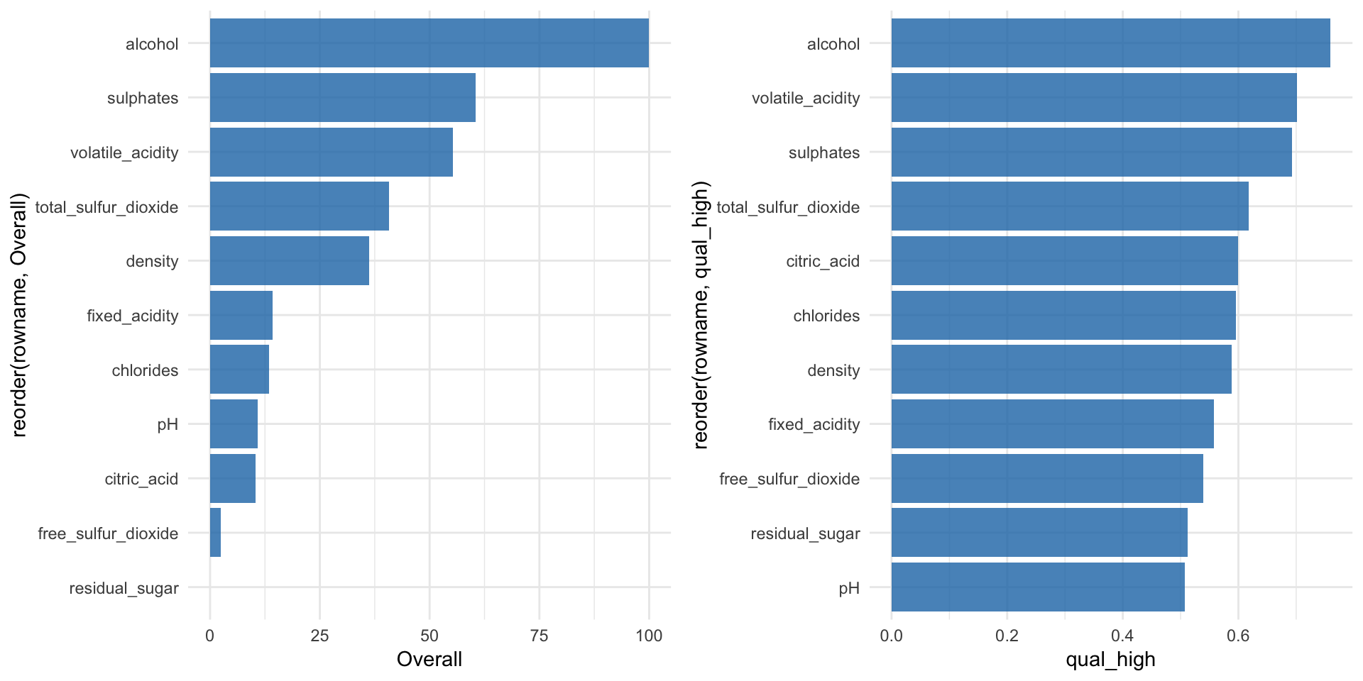
iml
The iml package combines a number of methods for explaining/interpreting machine learning model, like
- Feature importance
- Partial dependence plots
- Individual conditional expectation plots (ICE)
- Tree surrogate
- LocalModel: Local Interpretable Model-agnostic Explanations (similar to lime)
- Shapley value for explaining single predictions
In order to work with iml, we need to adapt our data a bit by removing the response variable and the creating a new predictor object that holds the model, the data and the class labels.
“The iml package uses R6 classes: New objects can be created by calling Predictor$new().” https://github.com/christophM/iml/blob/master/vignettes/intro.Rmd
X <- wine_train %>%
  select(-quality) %>%
  as.data.frame()

predictor <- Predictor$new(rf_model, data = X, y = wine_train$quality)
str(predictor)
## Classes 'Predictor', 'R6' <Predictor>
## Public:
## class: NULL
## clone: function (deep = FALSE)
## data: Data, R6
## initialize: function (model = NULL, data, predict.fun = NULL, y = NULL, class = NULL)
## model: train, train.formula
## predict: function (newdata)
## prediction.colnames: NULL
## prediction.function: function (newdata)
## print: function ()
## task: classification
## Private:
## predictionChecked: FALSEPartial Dependence & Individual Conditional Expectation plots (ICE)
Now we can explore some of the different methods. Let’s start with partial dependence plots as we had already looked into feature importance.
“Besides knowing which features were important, we are interested in how the features influence the predicted outcome. The Partial class implements partial dependence plots and individual conditional expectation curves. Each individual line represents the predictions (y-axis) for one data point when we change one of the features (e.g. ‘lstat’ on the x-axis). The highlighted line is the point-wise average of the individual lines and equals the partial dependence plot. The marks on the x-axis indicates the distribution of the ‘lstat’ feature, showing how relevant a region is for interpretation (little or no points mean that we should not over-interpret this region).” https://github.com/christophM/iml/blob/master/vignettes/intro.Rmd#partial-dependence
We can look at individual features, like the alcohol or pH and plot the curves:
pdp_obj <- Partial$new(predictor, feature = "alcohol")
pdp_obj$center(min(wine_train$alcohol))
glimpse(pdp_obj$results)
## Observations: 51,240
## Variables: 5
## $ alcohol <dbl> 8.400000, 8.742105, 9.084211, 9.426316, 9.768421, 10.1...
## $ .class <fct> qual_high, qual_high, qual_high, qual_high, qual_high,...
## $ .y.hat <dbl> 0.00000000, 0.00259375, -0.02496406, -0.03126250, 0.02...
## $ .type <chr> "pdp", "pdp", "pdp", "pdp", "pdp", "pdp", "pdp", "pdp"...
## $ .id <int> NA, NA, NA, NA, NA, NA, NA, NA, NA, NA, NA, NA, NA, NA...“The partial dependence plot calculates and plots the dependence of f(X) on a single or two features. It’s the aggregate of all individual conditional expectation curves, that describe how, for a single observation, the prediction changes when the feature changes.” iml help for
Partial
pdp_obj$plot()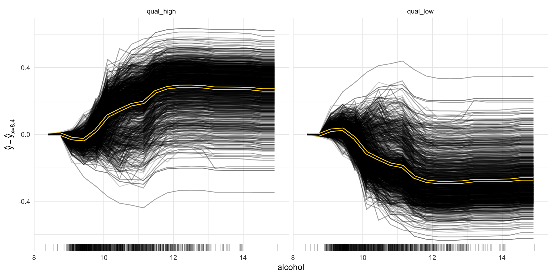
pdp_obj2 <- Partial$new(predictor, feature = c("sulphates", "pH"))
pdp_obj2$plot()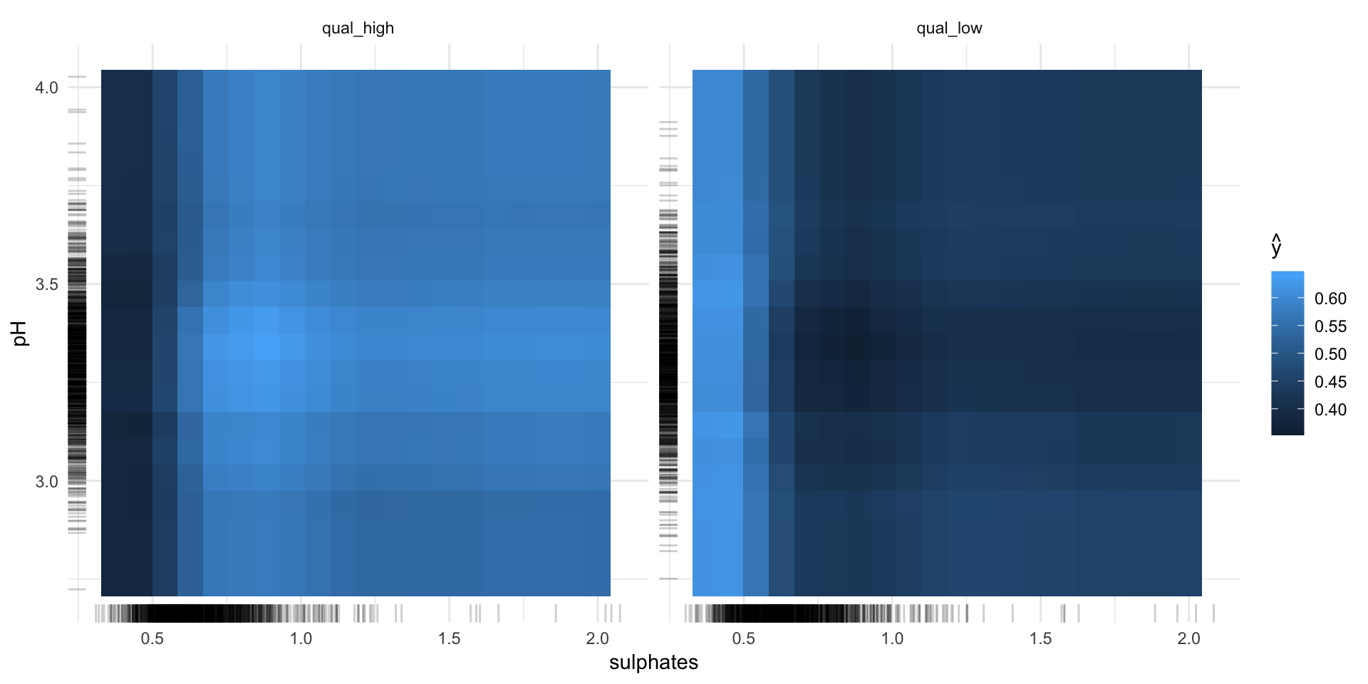
Feature interaction
“Interactions between features are measured via the decomposition of the prediction function: If a feature j has no interaction with any other feature, the prediction function can be expressed as the sum of the partial function that depends only on j and the partial function that only depends on features other than j. If the variance of the full function is completely explained by the sum of the partial functions, there is no interaction between feature j and the other features. Any variance that is not explained can be attributed to the interaction and is used as a measure of interaction strength. The interaction strength between two features is the proportion of the variance of the 2-dimensional partial dependence function that is not explained by the sum of the two 1-dimensional partial dependence functions. The interaction measure takes on values between 0 (no interaction) to 1.” iml help for
Interaction
interact <- Interaction$new(predictor, feature = "alcohol")All of these methods have a plot argument. However, since I am writing this for an article, I want all my plots to have the same look. That’s why I’m customizing the plots I want to use in my article as shown below.
#plot(interact)
interact$results %>%
  ggplot(aes(x = reorder(.feature, .interaction), y = .interaction, fill = .class)) +
    facet_wrap(~ .class, ncol = 2) +
    geom_bar(stat = "identity", alpha = 0.8) +
    scale_fill_tableau() +
    coord_flip() +
    guides(fill = FALSE)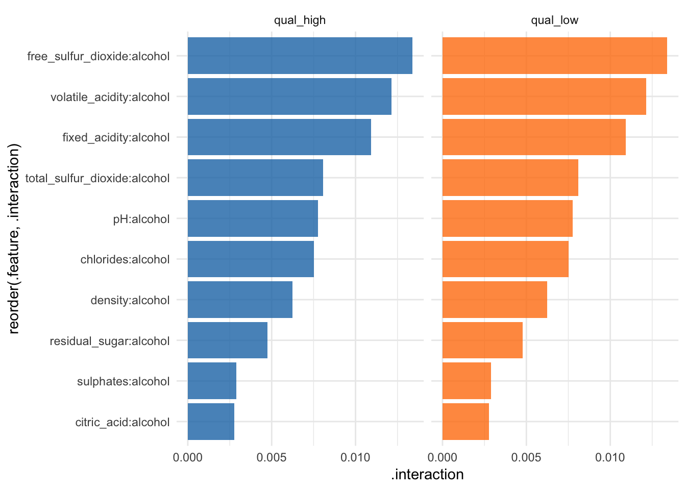
Tree Surrogate
The tree surrogate method uses decision trees on the predictions.
“A conditional inference tree is fitted on the predicted from the machine learning model and the data. The partykit package and function are used to fit the tree. By default a tree of maximum depth of 2 is fitted to improve interpretability.” iml help for
TreeSurrogate
tree <- TreeSurrogate$new(predictor, maxdepth = 5)The R^2 value gives an estimate of the goodness of fit or how well the decision tree approximates the model.
tree$r.squared## [1] 0.4571756 0.4571756#plot(tree)
tree$results %>%
mutate(prediction = colnames(select(., .y.hat.qual_high, .y.hat.qual_low))[max.col(select(., .y.hat.qual_high, .y.hat.qual_low),
ties.method = "first")],
prediction = ifelse(prediction == ".y.hat.qual_low", "qual_low", "qual_high")) %>%
ggplot(aes(x = prediction, fill = prediction)) +
facet_wrap(~ .path, ncol = 5) +
geom_bar(alpha = 0.8) +
scale_fill_tableau() +
guides(fill = FALSE)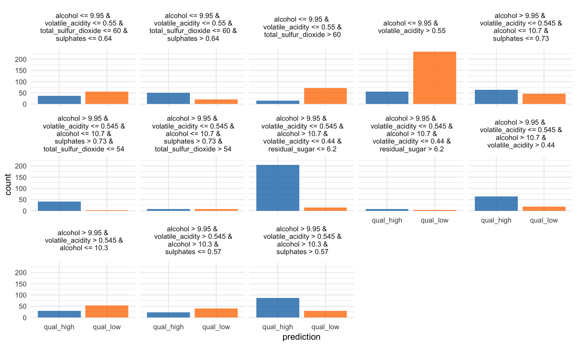
LocalModel: Local Interpretable Model-agnostic Explanations
LocalModel is a implementation of the LIME algorithm from Ribeiro et al. 2016, similar to lime.
According to the LIME principle, we can look at individual predictions. Here, for example on the first row of the test set:
X2 <- wine_test[, -12]
i = 1
lime_explain <- LocalModel$new(predictor, x.interest = X2[i, ])
lime_explain$results
## beta x.recoded effect x.original feature
## 1 -0.7653408409 0.7 -0.53573859 0.7 volatile_acidity
## 2 -0.0006292149 34.0 -0.02139331 34 total_sulfur_dioxide
## 3 0.2624431667 9.4 2.46696577 9.4 alcohol
## 4 0.7653408409 0.7 0.53573859 0.7 volatile_acidity
## 5 0.0006292149 34.0 0.02139331 34 total_sulfur_dioxide
## 6 -0.2624431667 9.4 -2.46696577 9.4 alcohol
## feature.value .class
## 1 volatile_acidity=0.7 qual_high
## 2 total_sulfur_dioxide=34 qual_high
## 3 alcohol=9.4 qual_high
## 4 volatile_acidity=0.7 qual_low
## 5 total_sulfur_dioxide=34 qual_low
## 6 alcohol=9.4 qual_low#plot(lime_explain)
p1 <- lime_explain$results %>%
ggplot(aes(x = reorder(feature.value, -effect), y = effect, fill = .class)) +
facet_wrap(~ .class, ncol = 2) +
geom_bar(stat = "identity", alpha = 0.8) +
scale_fill_tableau() +
coord_flip() +
labs(title = paste0("Test case #", i)) +
guides(fill = FALSE)… or for the sixth row:
i = 6
lime_explain$explain(X2[i, ])
p2 <- lime_explain$results %>%
  ggplot(aes(x = reorder(feature.value, -effect), y = effect, fill = .class)) +
    facet_wrap(~ .class, ncol = 2) +
    geom_bar(stat = "identity", alpha = 0.8) +
    scale_fill_tableau() +
    coord_flip() +
    labs(title = paste0("Test case #", i)) +
    guides(fill = FALSE)
grid.arrange(p1, p2, ncol = 2)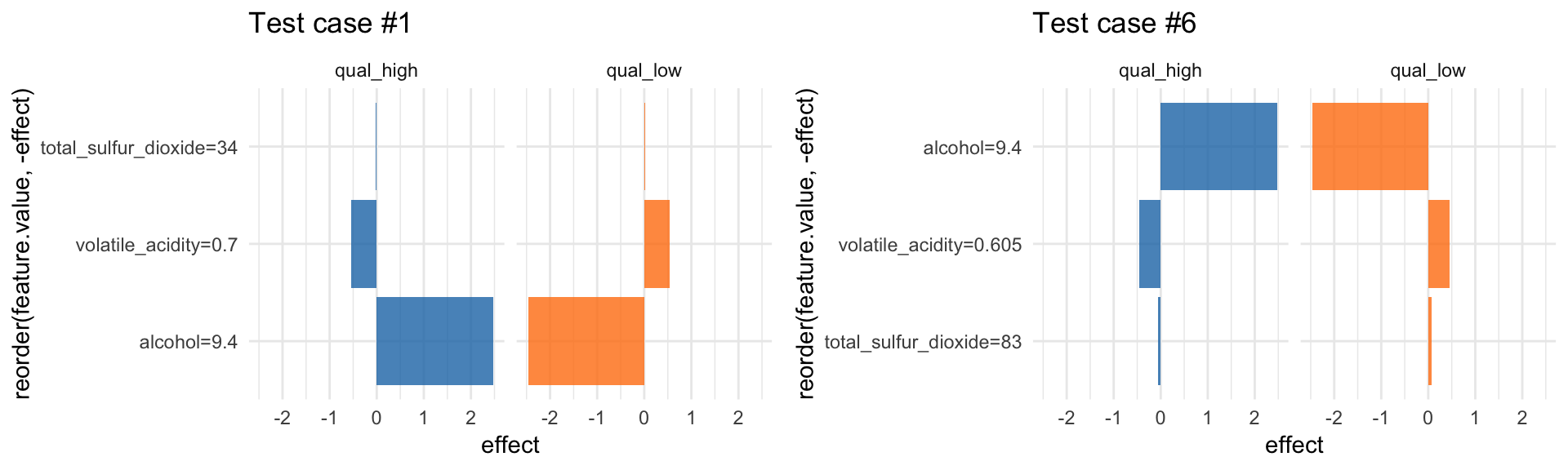
Shapley value for explaining single predictions
Another way to interpret individual predictions is whit Shapley values.
“Shapley computes feature contributions for single predictions with the Shapley value, an approach from cooperative game theory. The features values of an instance cooperate to achieve the prediction. The Shapley value fairly distributes the difference of the instance’s prediction and the datasets average prediction among the features.” iml help for
Shapley
More information about Shapley values can be found here.
shapley <- Shapley$new(predictor, x.interest = X2[1, ])head(shapley$results)## feature class phi phi.var
## 1 fixed_acidity qual_high -0.01100 0.003828485
## 2 volatile_acidity qual_high -0.16356 0.019123037
## 3 citric_acid qual_high -0.02318 0.005886472
## 4 residual_sugar qual_high -0.00950 0.001554939
## 5 chlorides qual_high -0.01580 0.002868889
## 6 free_sulfur_dioxide qual_high 0.00458 0.001250044
## feature.value
## 1 fixed_acidity=7.4
## 2 volatile_acidity=0.7
## 3 citric_acid=0
## 4 residual_sugar=1.9
## 5 chlorides=0.076
## 6 free_sulfur_dioxide=11#shapley$plot()
shapley$results %>%
ggplot(aes(x = reorder(feature.value, -phi), y = phi, fill = class)) +
facet_wrap(~ class, ncol = 2) +
geom_bar(stat = "identity", alpha = 0.8) +
scale_fill_tableau() +
coord_flip() +
guides(fill = FALSE)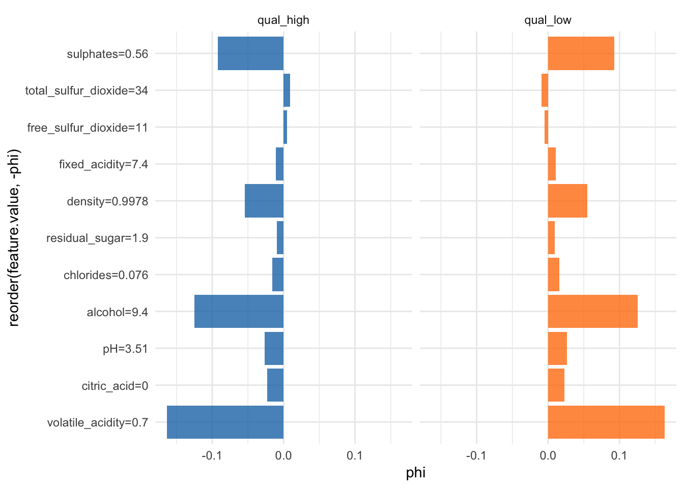
breakDown
Another package worth mentioning is breakDown. It provides
“Model agnostic tool for decomposition of predictions from black boxes. Break Down Table shows contributions of every variable to a final prediction. Break Down Plot presents variable contributions in a concise graphical way. This package work for binary classifiers and general regression models.” https://cran.r-project.org/web/packages/breakDown/index.html
The broken() function decomposes model predictions and outputs the contributions of each feature to the final prediction.
predict.function <- function(model, new_observation) {
  predict(model, new_observation, type="prob")[,2]
}
predict.function(rf_model, X2[1, ])
## [1] 0.966br <- broken(model = rf_model,
new_observation = X2[1, ],
data = X,
baseline = "Intercept",
predict.function = predict.function,
keep_distributions = TRUE)
br## contribution
## (Intercept) 0.000
## + alcohol = 9.4 0.138
## + volatile_acidity = 0.7 0.097
## + sulphates = 0.56 0.060
## + density = 0.9978 0.038
## + pH = 3.51 0.012
## + chlorides = 0.076 0.017
## + citric_acid = 0 0.026
## + fixed_acidity = 7.4 0.048
## + residual_sugar = 1.9 0.014
## + free_sulfur_dioxide = 11 0.016
## + total_sulfur_dioxide = 34 0.034
## final_prognosis 0.501
## baseline: 0.4654328The plot function shows the average predictions and the final prognosis:
#plot(br)
data.frame(y = br$contribution,
           x = br$variable) %>%
  ggplot(aes(x = reorder(x, y), y = y)) +
    geom_bar(stat = "identity", fill = "#1F77B4", alpha = 0.8) +
    coord_flip()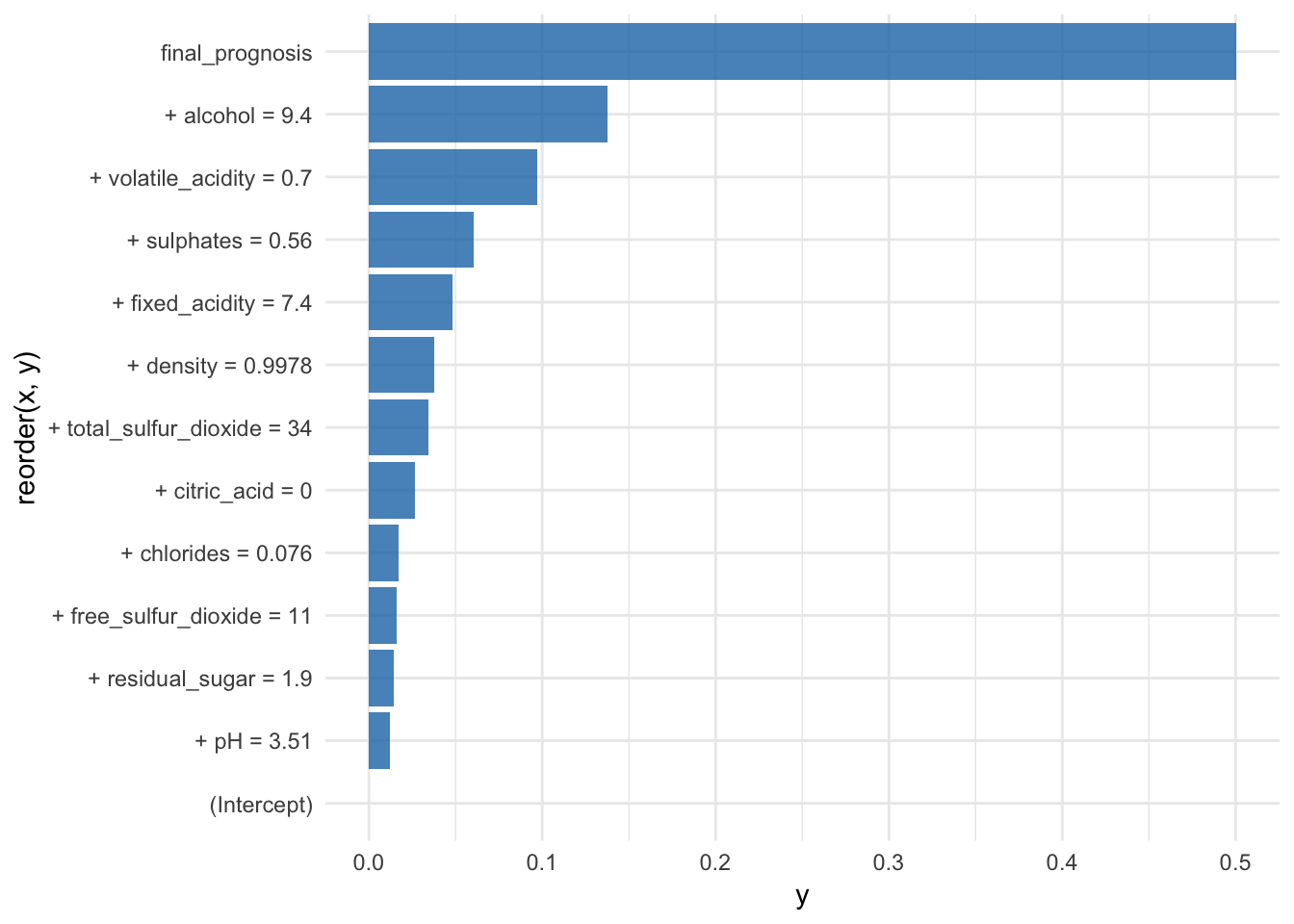
If we set keep_distributions = TRUE, we can plot these distributions of partial predictions, as well as the average.
plot(br, plot_distributions = TRUE)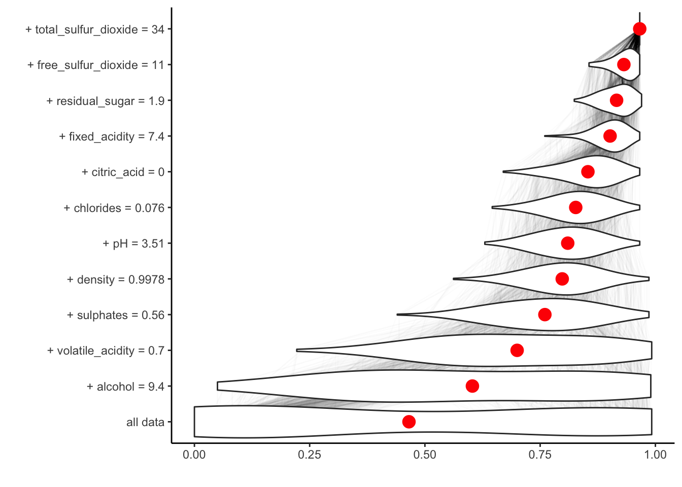
DALEX: Descriptive mAchine Learning EXplanations
The third package I want to showcase is DALEX, which stands for Descriptive mAchine Learning EXplanations and contains a collection of functions that help with interpreting/explaining black-box models.
“Machine Learning (ML) models are widely used and have various applications in classification or regression. Models created with boosting, bagging, stacking or similar techniques are often used due to their high performance, but such black-box models usually lack of interpretability. DALEX package contains various explainers that help to understand the link between input variables and model output. The single_variable() explainer extracts conditional response of a model as a function of a single selected variable. It is a wrapper over packages ‘pdp’ and ‘ALEPlot’. The single_prediction() explainer attributes parts of a model prediction to particular variables used in the model. It is a wrapper over ‘breakDown’ package. The variable_dropout() explainer calculates variable importance scores based on variable shuffling. All these explainers can be plotted with generic plot() function and compared across different models.” https://cran.r-project.org/web/packages/DALEX/index.html
We first create an explain object, that has the correct structure for use with the DALEX package.
p_fun <- function(object, newdata){predict(object, newdata = newdata, type = "prob")[, 2]}
yTest <- as.numeric(wine_test$quality)

explainer_classif_rf <- DALEX::explain(rf_model, label = "rf",
                                       data = wine_test, y = yTest,
                                       predict_function = p_fun)
Model performance
With DALEX we can do several things, for example analyze model performance as the distribution of residuals.
mp_classif_rf <- model_performance(explainer_classif_rf)plot(mp_classif_rf)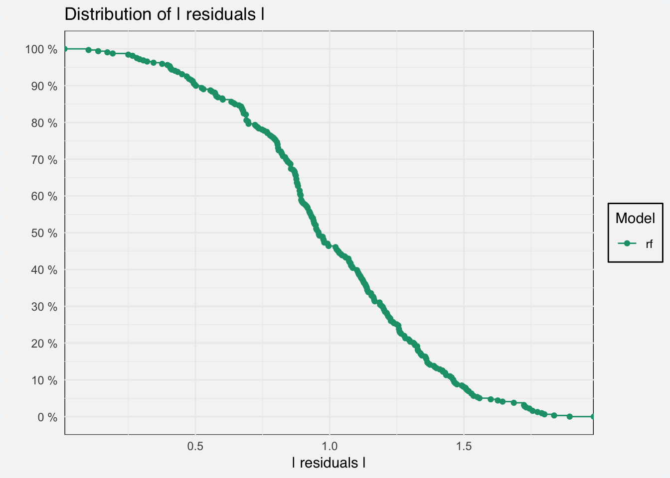
plot(mp_classif_rf, geom = "boxplot")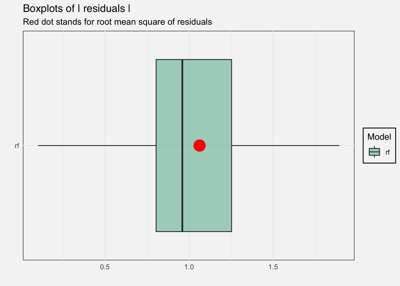
Feature importance
Feature importance can be measured with variable_importance() function, which gives the loss from variable dropout.
vi_classif_rf <- variable_importance(explainer_classif_rf, loss_function = loss_root_mean_square)plot(vi_classif_rf)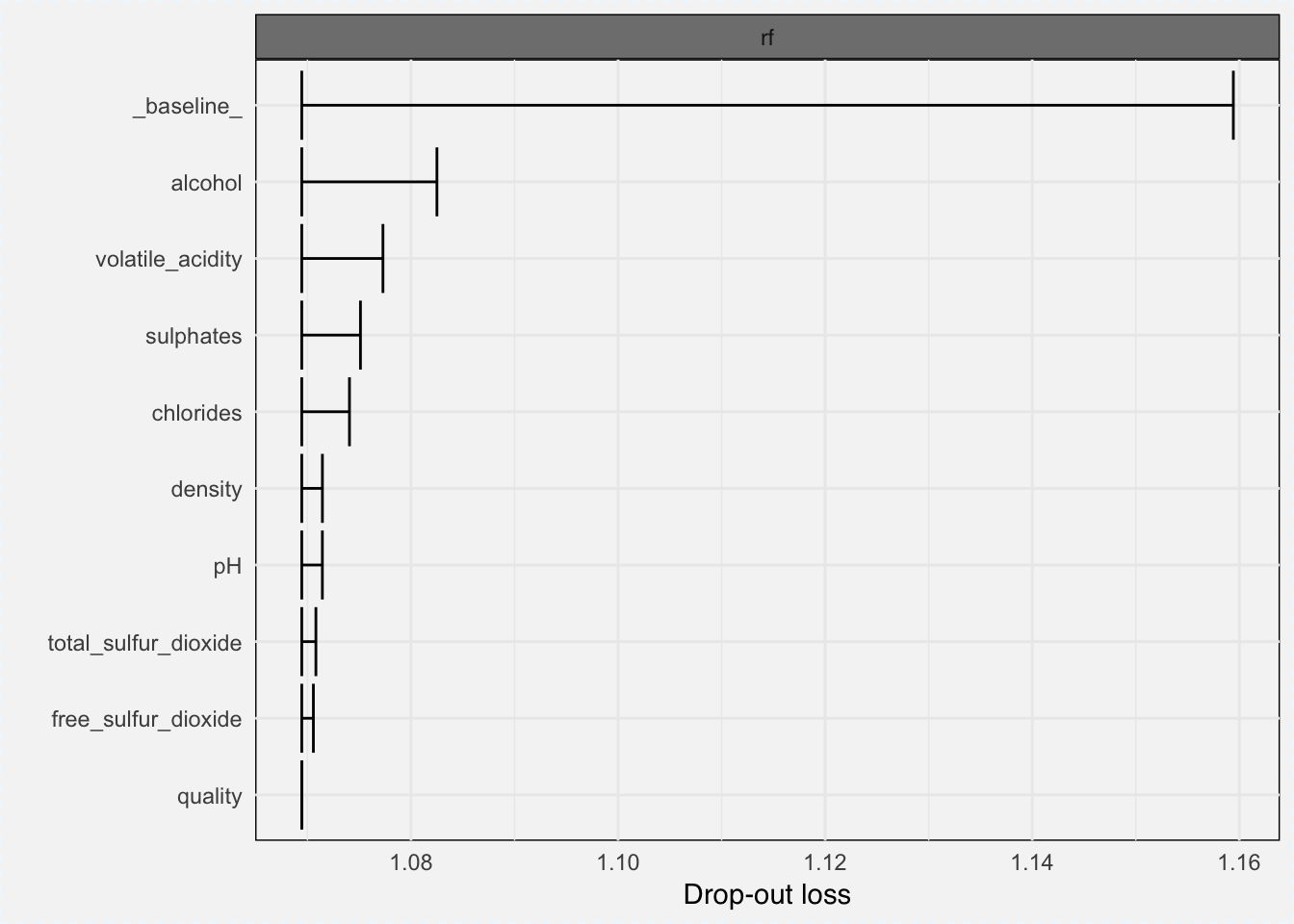
Variable response
And we can calculate the marginal response for a single variable with the variable_response() function.
“Calculates the average model response as a function of a single selected variable. Use the ‘type’ parameter to select the type of marginal response to be calculated. Currently for numeric variables we have Partial Dependency and Accumulated Local Effects implemented. Current implementation uses the ‘pdp’ package (Brandon M. Greenwell (2017). pdp: An R Package for Constructing Partial Dependence Plots. The R Journal, 9(1), 421–436.) and ‘ALEPlot’ (Dan Apley (2017). ALEPlot: Accumulated Local Effects Plots and Partial Dependence Plots.)” DALEX help for
variable_response
As type we can choose between ‘pdp’ for Partial Dependence Plots and ‘ale’ for Accumulated Local Effects.
pdp_classif_rf <- variable_response(explainer_classif_rf, variable = "alcohol", type = "pdp")plot(pdp_classif_rf)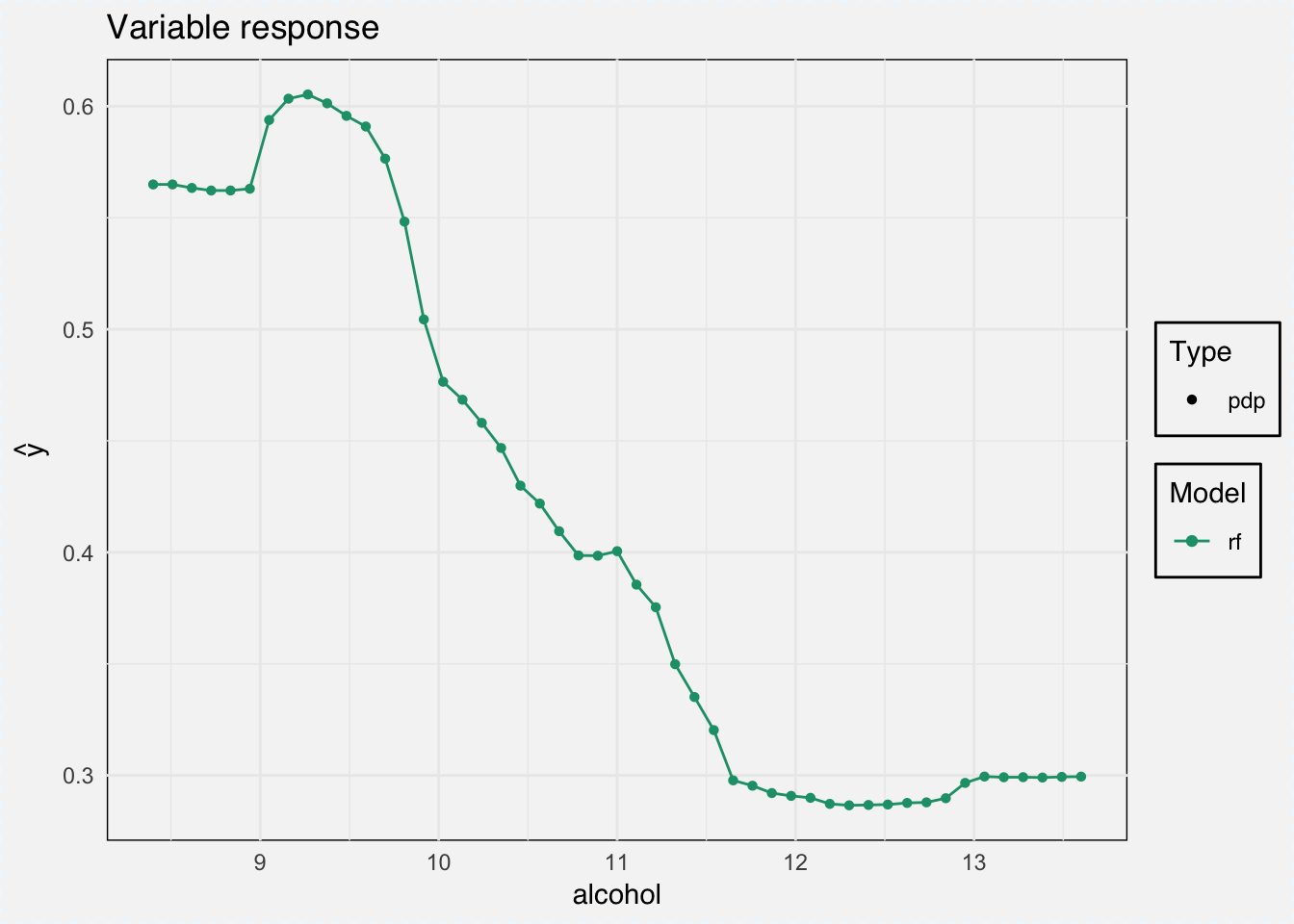
ale_classif_rf  <- variable_response(explainer_classif_rf, variable = "alcohol", type = "ale")
plot(ale_classif_rf)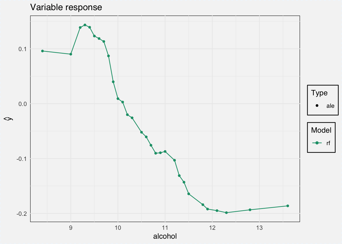
sessionInfo()## R version 3.5.1 (2018-07-02)
## Platform: x86_64-apple-darwin15.6.0 (64-bit)
## Running under: macOS High Sierra 10.13.6
##
## Matrix products: default
## BLAS: /Library/Frameworks/R.framework/Versions/3.5/Resources/lib/libRblas.0.dylib
## LAPACK: /Library/Frameworks/R.framework/Versions/3.5/Resources/lib/libRlapack.dylib
##
## locale:
## [1] de_DE.UTF-8/de_DE.UTF-8/de_DE.UTF-8/C/de_DE.UTF-8/de_DE.UTF-8
##
## attached base packages:
## [1] grid stats graphics grDevices utils datasets methods
## [8] base
##
## other attached packages:
## [1] gower_0.1.2 glmnet_2.0-16 foreach_1.4.4 Matrix_1.2-14
## [5] bindrcpp_0.2.2 DALEX_0.2.3 breakDown_0.1.6 iml_0.5.1
## [9] ggthemes_3.5.0 ggridges_0.5.0 gridExtra_2.3 caret_6.0-80
## [13] lattice_0.20-35 forcats_0.3.0 stringr_1.3.1 dplyr_0.7.6
## [17] purrr_0.2.5 readr_1.1.1 tidyr_0.8.1 tibble_1.4.2
## [21] ggplot2_3.0.0 tidyverse_1.2.1
##
## loaded via a namespace (and not attached):
## [1] readxl_1.1.0 backports_1.1.2 plyr_1.8.4
## [4] lazyeval_0.2.1 sp_1.3-1 splines_3.5.1
## [7] AlgDesign_1.1-7.3 digest_0.6.15 htmltools_0.3.6
## [10] gdata_2.18.0 magrittr_1.5 checkmate_1.8.5
## [13] cluster_2.0.7-1 sfsmisc_1.1-2 Metrics_0.1.4
## [16] recipes_0.1.3 modelr_0.1.2 dimRed_0.1.0
## [19] gmodels_2.18.1 colorspace_1.3-2 rvest_0.3.2
## [22] haven_1.1.2 xfun_0.3 crayon_1.3.4
## [25] jsonlite_1.5 libcoin_1.0-1 ALEPlot_1.1
## [28] bindr_0.1.1 survival_2.42-3 iterators_1.0.9
## [31] glue_1.2.0 DRR_0.0.3 gtable_0.2.0
## [34] ipred_0.9-6 questionr_0.6.2 kernlab_0.9-26
## [37] ddalpha_1.3.4 DEoptimR_1.0-8 abind_1.4-5
## [40] scales_0.5.0 mvtnorm_1.0-8 miniUI_0.1.1.1
## [43] Rcpp_0.12.17 xtable_1.8-2 spData_0.2.9.0
## [46] magic_1.5-8 proxy_0.4-22 foreign_0.8-70
## [49] spdep_0.7-7 Formula_1.2-3 stats4_3.5.1
## [52] lava_1.6.2 prodlim_2018.04.18 httr_1.3.1
## [55] yaImpute_1.0-29 RColorBrewer_1.1-2 pkgconfig_2.0.1
## [58] nnet_7.3-12 deldir_0.1-15 labeling_0.3
## [61] tidyselect_0.2.4 rlang_0.2.1 reshape2_1.4.3
## [64] later_0.7.3 munsell_0.5.0 cellranger_1.1.0
## [67] tools_3.5.1 cli_1.0.0 factorMerger_0.3.6
## [70] pls_2.6-0 broom_0.4.5 evaluate_0.10.1
## [73] geometry_0.3-6 yaml_2.1.19 ModelMetrics_1.1.0
## [76] knitr_1.20 robustbase_0.93-1 pdp_0.6.0
## [79] randomForest_4.6-14 nlme_3.1-137 mime_0.5
## [82] RcppRoll_0.3.0 xml2_1.2.0 compiler_3.5.1
## [85] rstudioapi_0.7 e1071_1.6-8 klaR_0.6-14
## [88] stringi_1.2.3 highr_0.7 blogdown_0.6
## [91] psych_1.8.4 pillar_1.2.3 LearnBayes_2.15.1
## [94] combinat_0.0-8 data.table_1.11.4 httpuv_1.4.4.2
## [97] agricolae_1.2-8 R6_2.2.2 bookdown_0.7
## [100] promises_1.0.1 codetools_0.2-15 boot_1.3-20
## [103] MASS_7.3-50 gtools_3.8.1 assertthat_0.2.0
## [106] CVST_0.2-2 rprojroot_1.3-2 withr_2.1.2
## [109] mnormt_1.5-5 expm_0.999-2 parallel_3.5.1
## [112] hms_0.4.2 rpart_4.1-13 timeDate_3043.102
## [115] coda_0.19-1 class_7.3-14 rmarkdown_1.10
## [118] inum_1.0-0 ggpubr_0.1.7 partykit_1.2-2
## [121] shiny_1.1.0 lubridate_1.7.4