
Explaining Black-Box Machine Learning Models - Code Part 2: Text classification with LIME
This is code that will encompany an article that will appear in a special edition of a German IT magazine. The article is about explaining black-box machine learning models. In that article I’m showcasing three practical examples:
- Explaining supervised classification models built on tabular data using
caretand theimlpackage - Explaining image classification models with
kerasandlime - Explaining text classification models with
xgboostandlime
Below, you will find the code for the third part: Text classification with lime.
# data wrangling
library(tidyverse)
library(readr)

# plotting
library(ggthemes)
theme_set(theme_minimal())

# text prep
library(text2vec)

# ml
library(caret)
library(xgboost)

# explanation
library(lime)
Text classification models
Here I am using another Kaggle dataset: Women’s e-commerce cloting reviews. The data contains a text review of different items of clothing, as well as some additional information, like rating, division, etc.
In this example, I will use the review title and text in order to classify whether or not the item was liked. I am creating the response variable from the rating: every item rates with 5 stars is considered “liked” (1), the rest as “not liked” (0). I am also combining review title and text.
clothing_reviews <- read_csv("/Users/shiringlander/Documents/Github/ix_lime_etc/Womens Clothing E-Commerce Reviews.csv") %>%
  mutate(Liked = as.factor(ifelse(Rating == 5, 1, 0)),
         text = paste(Title, `Review Text`),
         text = gsub("NA", "", text))
## Parsed with column specification:
## cols(
## X1 = col_integer(),
## `Clothing ID` = col_integer(),
## Age = col_integer(),
## Title = col_character(),
## `Review Text` = col_character(),
## Rating = col_integer(),
## `Recommended IND` = col_integer(),
## `Positive Feedback Count` = col_integer(),
## `Division Name` = col_character(),
## `Department Name` = col_character(),
## `Class Name` = col_character()
## )glimpse(clothing_reviews)## Observations: 23,486
## Variables: 13
## $ X1 <int> 0, 1, 2, 3, 4, 5, 6, 7, 8, 9, 10, 11...
## $ `Clothing ID` <int> 767, 1080, 1077, 1049, 847, 1080, 85...
## $ Age <int> 33, 34, 60, 50, 47, 49, 39, 39, 24, ...
## $ Title <chr> NA, NA, "Some major design flaws", "...
## $ `Review Text` <chr> "Absolutely wonderful - silky and se...
## $ Rating <int> 4, 5, 3, 5, 5, 2, 5, 4, 5, 5, 3, 5, ...
## $ `Recommended IND` <int> 1, 1, 0, 1, 1, 0, 1, 1, 1, 1, 0, 1, ...
## $ `Positive Feedback Count` <int> 0, 4, 0, 0, 6, 4, 1, 4, 0, 0, 14, 2,...
## $ `Division Name` <chr> "Initmates", "General", "General", "...
## $ `Department Name` <chr> "Intimate", "Dresses", "Dresses", "B...
## $ `Class Name` <chr> "Intimates", "Dresses", "Dresses", "...
## $ Liked <fct> 0, 1, 0, 1, 1, 0, 1, 0, 1, 1, 0, 1, ...
## $ text <chr> " Absolutely wonderful - silky and s...Whether an item was liked or not will thus be my response variable or label for classification.
clothing_reviews %>%
  ggplot(aes(x = Liked, fill = Liked)) +
    geom_bar(alpha = 0.8) +
    scale_fill_tableau(palette = "tableau20") +
    guides(fill = FALSE)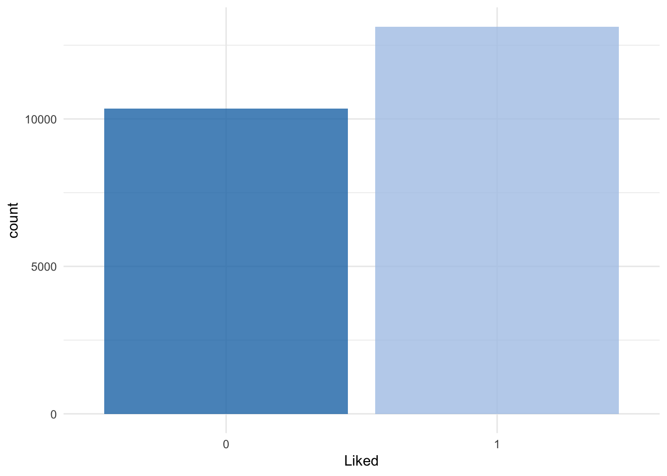
Let’s split the data into train and test sets:
set.seed(42)
idx <- createDataPartition(clothing_reviews$Liked,
                           p = 0.8,
                           list = FALSE,
                           times = 1)

clothing_reviews_train <- clothing_reviews[ idx,]
clothing_reviews_test  <- clothing_reviews[-idx,]
Let’s start simple
The first text model I’m looking at has been built similarly to the example model in the help for lime::interactive_text_explanations().
First, we need to prepare the data for modeling: we will need to convert the text to a document term matrix (dtm). There are different ways to do this. One is be with the text2vec package.
“Because of R’s copy-on-modify semantics, it is not easy to iteratively grow a DTM. Thus constructing a DTM, even for a small collections of documents, can be a serious bottleneck for analysts and researchers. It involves reading the whole collection of text documents into RAM and processing it as single vector, which can easily increase memory use by a factor of 2 to 4. The text2vec package solves this problem by providing a better way of constructing a document-term matrix.” https://cran.r-project.org/web/packages/text2vec/vignettes/text-vectorization.html
Alternatives to text2vec would be tm + SnowballC or you could work with the tidytext package.
The itoken() function creates vocabularies (here stemmed words), from which we can create the dtm with the create_dtm() function.
All preprocessing steps, starting from the raw text, need to be wrapped in a function that can then be pasted into the lime::lime() function; this is only necessary if you want to use your model with lime.
get_matrix <- function(text) {
  it <- itoken(text, progressbar = FALSE)
  create_dtm(it, vectorizer = hash_vectorizer())
}
Now, this preprocessing function can be applied to both training and test data.
dtm_train <- get_matrix(clothing_reviews_train$text)
str(dtm_train)
## Formal class 'dgCMatrix' [package "Matrix"] with 6 slots
## ..@ i : int [1:889012] 304 764 786 788 793 794 1228 2799 2819 3041 ...
## ..@ p : int [1:262145] 0 0 0 0 0 0 0 0 0 0 ...
## ..@ Dim : int [1:2] 18789 262144
## ..@ Dimnames:List of 2
## .. ..$ : chr [1:18789] "1" "2" "3" "4" ...
## .. ..$ : NULL
## ..@ x : num [1:889012] 1 1 2 1 2 1 1 1 1 1 ...
## ..@ factors : list()dtm_test <- get_matrix(clothing_reviews_test$text)
str(dtm_test)## Formal class 'dgCMatrix' [package "Matrix"] with 6 slots
## ..@ i : int [1:222314] 2793 400 477 622 2818 2997 3000 4500 3524 2496 ...
## ..@ p : int [1:262145] 0 0 0 0 0 0 0 0 0 0 ...
## ..@ Dim : int [1:2] 4697 262144
## ..@ Dimnames:List of 2
## .. ..$ : chr [1:4697] "1" "2" "3" "4" ...
## .. ..$ : NULL
## ..@ x : num [1:222314] 1 1 1 1 1 1 1 1 1 1 ...
## ..@ factors : list()And we use it to train a model with the xgboost package (just as in the example of the lime package).
xgb_model <- xgb.train(list(max_depth = 7,
                            eta = 0.1,
                            objective = "binary:logistic",
                            eval_metric = "error", nthread = 1),
                       xgb.DMatrix(dtm_train,
                                   label = clothing_reviews_train$Liked == "1"),
                       nrounds = 50)
Let’s try it on the test data and see how it performs:
pred <- predict(xgb_model, dtm_test)

confusionMatrix(clothing_reviews_test$Liked,
                as.factor(round(pred, digits = 0)))
## Confusion Matrix and Statistics
##
## Reference
## Prediction 0 1
## 0 1370 701
## 1 421 2205
##
## Accuracy : 0.7611
## 95% CI : (0.7487, 0.7733)
## No Information Rate : 0.6187
## P-Value [Acc > NIR] : < 2.2e-16
##
## Kappa : 0.5085
## Mcnemar's Test P-Value : < 2.2e-16
##
## Sensitivity : 0.7649
## Specificity : 0.7588
## Pos Pred Value : 0.6615
## Neg Pred Value : 0.8397
## Prevalence : 0.3813
## Detection Rate : 0.2917
## Detection Prevalence : 0.4409
## Balanced Accuracy : 0.7619
##
## 'Positive' Class : 0
## Okay, not a perfect score but good enough for me - right now, I’m more interested in the explanations of the model’s predictions. For this, we need to run the lime() function and give it
- the text input that was used to construct the model
- the trained model
- the preprocessing function
explainer <- lime(clothing_reviews_train$text,
                  xgb_model,
                  preprocess = get_matrix)
With this, we could right away call the interactive explainer Shiny app, where we can type any text we want into the field on the left and see the explanation on the right: words that are underlined green support the classification, red words contradict them.
interactive_text_explanations(explainer)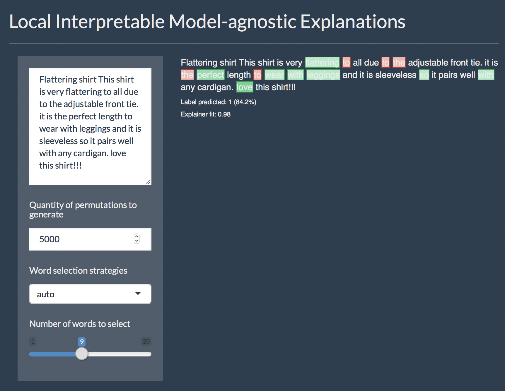
What happens in the background in the app, we can do explicitly by calling the explain() function and give it
- the test data (here the first four reviews of the test set)
- the explainer defined with the
lime()function - the number of labels we want to have explanations for (alternatively, you set the label by name)
- and the number of features (in this case words) that should be included in the explanations
We can plot them either with the plot_text_explanations() function, which gives an output like in the Shiny app or we use the regular plot_features() function.
explanations <- lime::explain(clothing_reviews_test$text[1:4], explainer, n_labels = 1, n_features = 5)plot_text_explanations(explanations)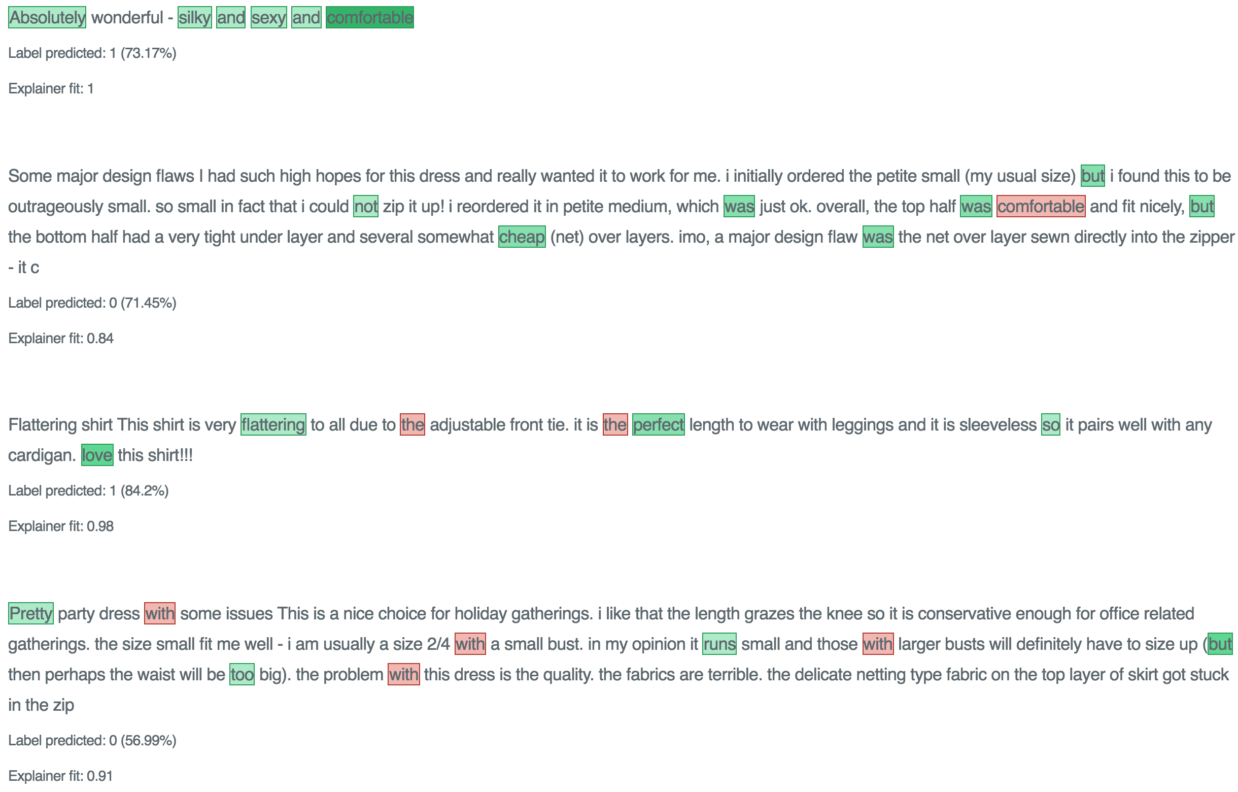
plot_features(explanations)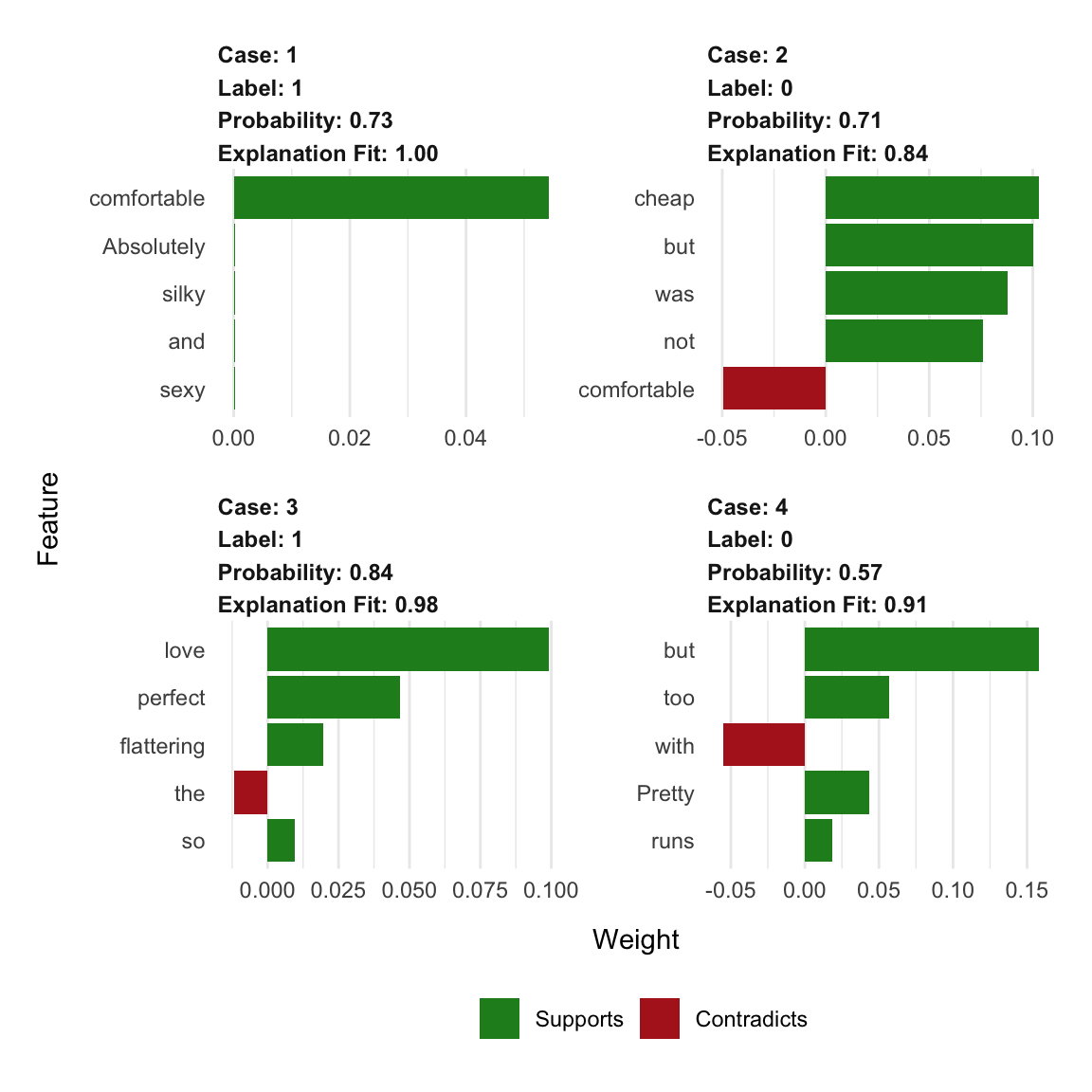
As we can see, our explanations contain a lot of stop-words that don’t really make much sense as features in our model. So…
… let’s try a more complex example
Okay, our model above works but there are still common words and stop words in our model that LIME picks up on. Ideally, we would want to remove them before modeling and keep only relevant words. This we can accomplish by using additional steps and options in our preprocessing function.
Important to know is that whatever preprocessing we do with our text corpus, train and test data has to have the same features (i.e. words)! If we were to incorporate all the steps shown below into one function and call it separately on train and test data, we would end up with different words in our dtm and the predict() function won’t work any more. In the simple example above, it works because we have been using the hash_vectorizer().
Nevertheless, the lime::explain() function expects a preprocessing function that takes a character vector as input.
How do we go about this? First, we will need to create the vocabulary just from the training data. To reduce the number of words to only the most relevant I am performing the following steps:
- stem all words
- remove step-words
- prune vocabulary
- transform into vector space
stem_tokenizer <- function(x) {
  lapply(word_tokenizer(x),
         SnowballC::wordStem,
         language = "en")
}

stop_words = tm::stopwords(kind = "en")

# create prunded vocabulary
vocab_train <- itoken(clothing_reviews_train$text,
                     preprocess_function = tolower,
                     tokenizer = stem_tokenizer,
                     progressbar = FALSE)

v <- create_vocabulary(vocab_train,
                       stopwords = stop_words)

pruned_vocab <- prune_vocabulary(v,
                                  doc_proportion_max = 0.99,
                                  doc_proportion_min = 0.01)

vectorizer_train <- vocab_vectorizer(pruned_vocab)
This vector space can now be added to the preprocessing function, which we can then apply to both train and test data. Here, I am also transforming the word counts to tfidf values.
# preprocessing function
create_dtm_mat <- function(text, vectorizer = vectorizer_train) {

  vocab <- itoken(text,
               preprocess_function = tolower,
               tokenizer = stem_tokenizer,
               progressbar = FALSE)

  dtm <- create_dtm(vocab,
             vectorizer = vectorizer)

  tfidf = TfIdf$new()
  fit_transform(dtm, tfidf)
}
dtm_train2 <- create_dtm_mat(clothing_reviews_train$text)
str(dtm_train2)## Formal class 'dgCMatrix' [package "Matrix"] with 6 slots
## ..@ i : int [1:415770] 26 74 169 294 588 693 703 708 727 759 ...
## ..@ p : int [1:506] 0 189 380 574 765 955 1151 1348 1547 1740 ...
## ..@ Dim : int [1:2] 18789 505
## ..@ Dimnames:List of 2
## .. ..$ : chr [1:18789] "1" "2" "3" "4" ...
## .. ..$ : chr [1:505] "ad" "sandal" "depend" "often" ...
## ..@ x : num [1:415770] 0.177 0.135 0.121 0.17 0.131 ...
## ..@ factors : list()dtm_test2 <- create_dtm_mat(clothing_reviews_test$text)
str(dtm_test2)## Formal class 'dgCMatrix' [package "Matrix"] with 6 slots
## ..@ i : int [1:103487] 228 304 360 406 472 518 522 624 732 784 ...
## ..@ p : int [1:506] 0 53 113 151 186 216 252 290 323 360 ...
## ..@ Dim : int [1:2] 4697 505
## ..@ Dimnames:List of 2
## .. ..$ : chr [1:4697] "1" "2" "3" "4" ...
## .. ..$ : chr [1:505] "ad" "sandal" "depend" "often" ...
## ..@ x : num [1:103487] 0.263 0.131 0.135 0.109 0.179 ...
## ..@ factors : list()And we will train another gradient boosting model:
xgb_model2 <- xgb.train(params = list(max_depth = 10,
                            eta = 0.2,
                            objective = "binary:logistic",
                            eval_metric = "error", nthread = 1),
                       data = xgb.DMatrix(dtm_train2,
                                   label = clothing_reviews_train$Liked == "1"),
                       nrounds = 500)
pred2 <- predict(xgb_model2, dtm_test2)
confusionMatrix(clothing_reviews_test$Liked,
as.factor(round(pred2, digits = 0)))## Confusion Matrix and Statistics
##
## Reference
## Prediction 0 1
## 0 1441 630
## 1 426 2200
##
## Accuracy : 0.7752
## 95% CI : (0.763, 0.787)
## No Information Rate : 0.6025
## P-Value [Acc > NIR] : < 2.2e-16
##
## Kappa : 0.5392
## Mcnemar's Test P-Value : 4.187e-10
##
## Sensitivity : 0.7718
## Specificity : 0.7774
## Pos Pred Value : 0.6958
## Neg Pred Value : 0.8378
## Prevalence : 0.3975
## Detection Rate : 0.3068
## Detection Prevalence : 0.4409
## Balanced Accuracy : 0.7746
##
## 'Positive' Class : 0
## Unfortunately, this didn’t really improve the classification accuracy but let’s look at the explanations again:
explainer2 <- lime(clothing_reviews_train$text,
                  xgb_model2,
                  preprocess = create_dtm_mat)
explanations2 <- lime::explain(clothing_reviews_test$text[1:4], explainer2, n_labels = 1, n_features = 4)
plot_text_explanations(explanations2)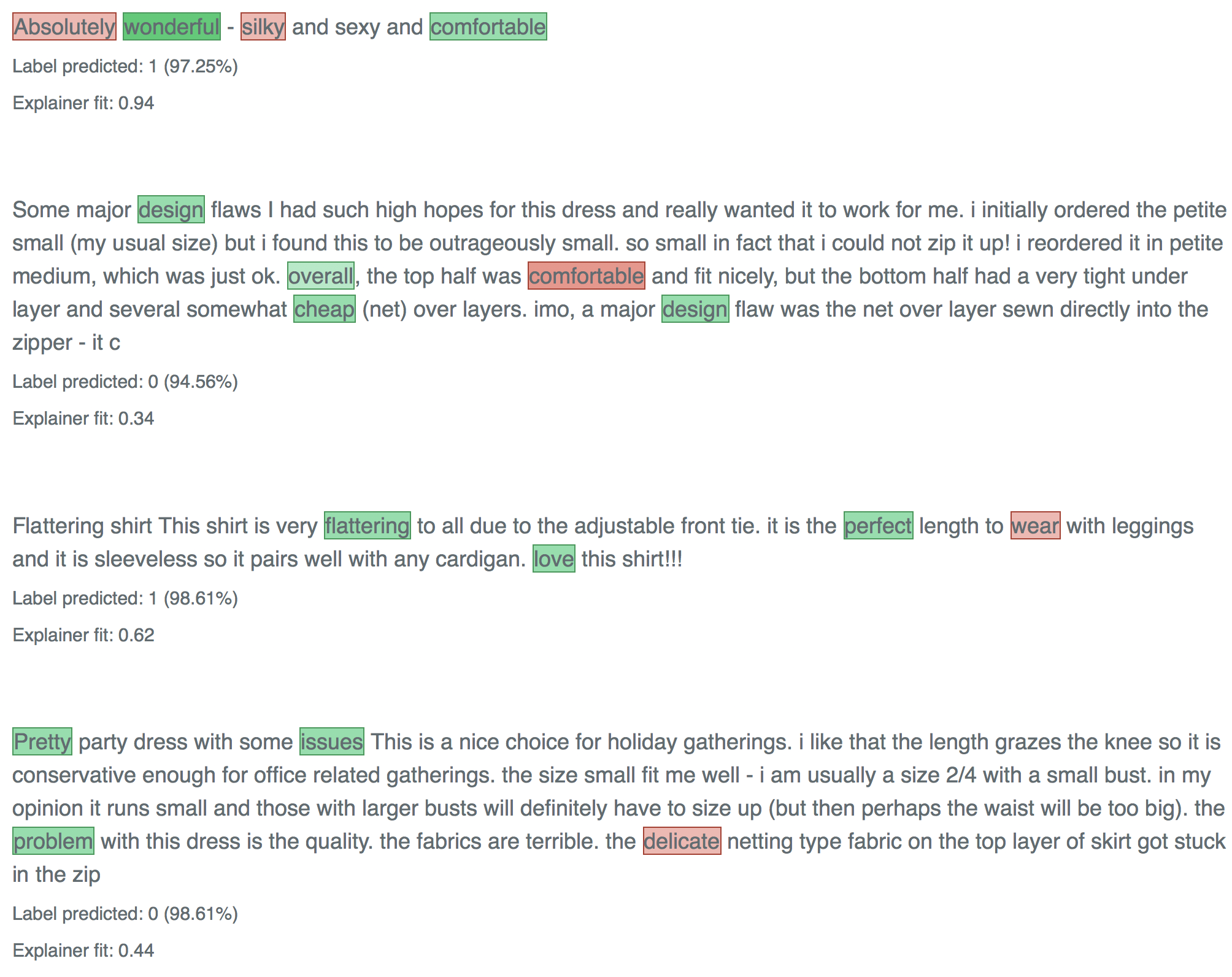
The words that get picked up now make much more sense! So, even though making my model more complex didn’t improve “the numbers”, this second model is likely to be much better able to generalize to new reviews because it seems to pick up on words that make intuitive sense.
That’s why I’m sold on the benefits of adding explainer functions to most machine learning workflows - and why I love the lime package in R!
sessionInfo()## R version 3.5.1 (2018-07-02)
## Platform: x86_64-apple-darwin15.6.0 (64-bit)
## Running under: macOS High Sierra 10.13.6
##
## Matrix products: default
## BLAS: /Library/Frameworks/R.framework/Versions/3.5/Resources/lib/libRblas.0.dylib
## LAPACK: /Library/Frameworks/R.framework/Versions/3.5/Resources/lib/libRlapack.dylib
##
## locale:
## [1] de_DE.UTF-8/de_DE.UTF-8/de_DE.UTF-8/C/de_DE.UTF-8/de_DE.UTF-8
##
## attached base packages:
## [1] stats graphics grDevices utils datasets methods base
##
## other attached packages:
## [1] bindrcpp_0.2.2 lime_0.4.0 xgboost_0.71.2 caret_6.0-80
## [5] lattice_0.20-35 text2vec_0.5.1 ggthemes_3.5.0 forcats_0.3.0
## [9] stringr_1.3.1 dplyr_0.7.6 purrr_0.2.5 readr_1.1.1
## [13] tidyr_0.8.1 tibble_1.4.2 ggplot2_3.0.0 tidyverse_1.2.1
##
## loaded via a namespace (and not attached):
## [1] colorspace_1.3-2 class_7.3-14 rprojroot_1.3-2
## [4] futile.logger_1.4.3 pls_2.6-0 rstudioapi_0.7
## [7] DRR_0.0.3 SnowballC_0.5.1 prodlim_2018.04.18
## [10] lubridate_1.7.4 xml2_1.2.0 codetools_0.2-15
## [13] splines_3.5.1 mnormt_1.5-5 robustbase_0.93-1
## [16] knitr_1.20 shinythemes_1.1.1 RcppRoll_0.3.0
## [19] mlapi_0.1.0 jsonlite_1.5 broom_0.4.5
## [22] ddalpha_1.3.4 kernlab_0.9-26 sfsmisc_1.1-2
## [25] shiny_1.1.0 compiler_3.5.1 httr_1.3.1
## [28] backports_1.1.2 assertthat_0.2.0 Matrix_1.2-14
## [31] lazyeval_0.2.1 cli_1.0.0 later_0.7.3
## [34] formatR_1.5 htmltools_0.3.6 tools_3.5.1
## [37] NLP_0.1-11 gtable_0.2.0 glue_1.2.0
## [40] reshape2_1.4.3 Rcpp_0.12.17 slam_0.1-43
## [43] cellranger_1.1.0 nlme_3.1-137 blogdown_0.6
## [46] iterators_1.0.9 psych_1.8.4 timeDate_3043.102
## [49] gower_0.1.2 xfun_0.3 rvest_0.3.2
## [52] mime_0.5 stringdist_0.9.5.1 DEoptimR_1.0-8
## [55] MASS_7.3-50 scales_0.5.0 ipred_0.9-6
## [58] hms_0.4.2 promises_1.0.1 parallel_3.5.1
## [61] lambda.r_1.2.3 yaml_2.1.19 rpart_4.1-13
## [64] stringi_1.2.3 foreach_1.4.4 e1071_1.6-8
## [67] lava_1.6.2 geometry_0.3-6 rlang_0.2.1
## [70] pkgconfig_2.0.1 evaluate_0.10.1 bindr_0.1.1
## [73] labeling_0.3 recipes_0.1.3 htmlwidgets_1.2
## [76] CVST_0.2-2 tidyselect_0.2.4 plyr_1.8.4
## [79] magrittr_1.5 bookdown_0.7 R6_2.2.2
## [82] magick_1.9 dimRed_0.1.0 pillar_1.2.3
## [85] haven_1.1.2 foreign_0.8-70 withr_2.1.2
## [88] survival_2.42-3 abind_1.4-5 nnet_7.3-12
## [91] modelr_0.1.2 crayon_1.3.4 futile.options_1.0.1
## [94] rmarkdown_1.10 grid_3.5.1 readxl_1.1.0
## [97] data.table_1.11.4 ModelMetrics_1.1.0 digest_0.6.15
## [100] tm_0.7-4 xtable_1.8-2 httpuv_1.4.4.2
## [103] RcppParallel_4.4.0 stats4_3.5.1 munsell_0.5.0
## [106] glmnet_2.0-16 magic_1.5-8