How do Convolutional Neural Nets (CNNs) learn? + Keras example

Convolutional Neural Nets

Convolutional Neural Nets are usually abbreviated either CNNs or ConvNets. They are a specific type of neural network that has very particular differences compared to MLPs. Basically, you can think of CNNs as working similarly to the receptive fields of photoreceptors in the human eye. Receptive fields in our eyes are small connected areas on the retina where groups of many photo-receptors stimulate much fewer ganglion cells. Thus, each ganglion cell can be stimulated by a large number of receptors, so that a complex input is condensed into a compressed output before it is further processed in the brain.

How does a computer see images

Before we dive deeper into CNNs, I briefly want to recap how images can take on a numerical format. We need a numerical representation of our image because just like any other machine learning model or neural net, CNNs need data in form of numbers in order to learn! With images, these numbers are pixel values; when we have a grey-scale image, these values represent a range of “greyness” from 0 (black) to 255 (white).

Here is an example image from the fruits datasets, which is used in the practical example for this lesson. In general, data can be represented in different formats, e.g. as vectors, tables or matrices. I am using the imager package to read the image and have a look at the pixel values, which are represented as a matrix with the dimensions image width x image height.

library(imager)
im <- load.image("/Users/shiringlander/Documents/Github/codecentric.AI-bootcamp/data/fruits-360/Training/Strawberry/100_100.jpg")

plot(im)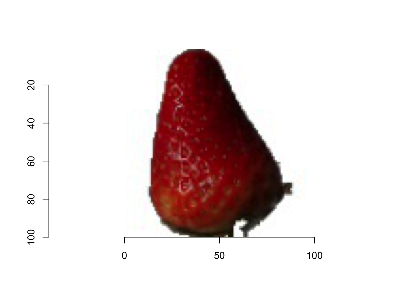

But when we look at the dim() function with our image, we see that there are actually four dimensions and only the first two represent image width and image height. The third dimension is for the depth, which means in case of videos the time or order of the frames; with regular images, we don’t need this dimension. The third dimension shows the number of color channels; in this case, we have a color image, so there are three channels for red, green and blue. The values remain in the same between 0 and 255 but now they don’t represent grey-scales but color intensity of the respective channel. This 3-dimensional format (a stack of three matrices) is also called a 3-dimensional array.

dim(im)

## [1] 100 100   1   3

Let’s see what happens if we convert our image to greyscale:

im_grey <- grayscale(im)
plot(im_grey)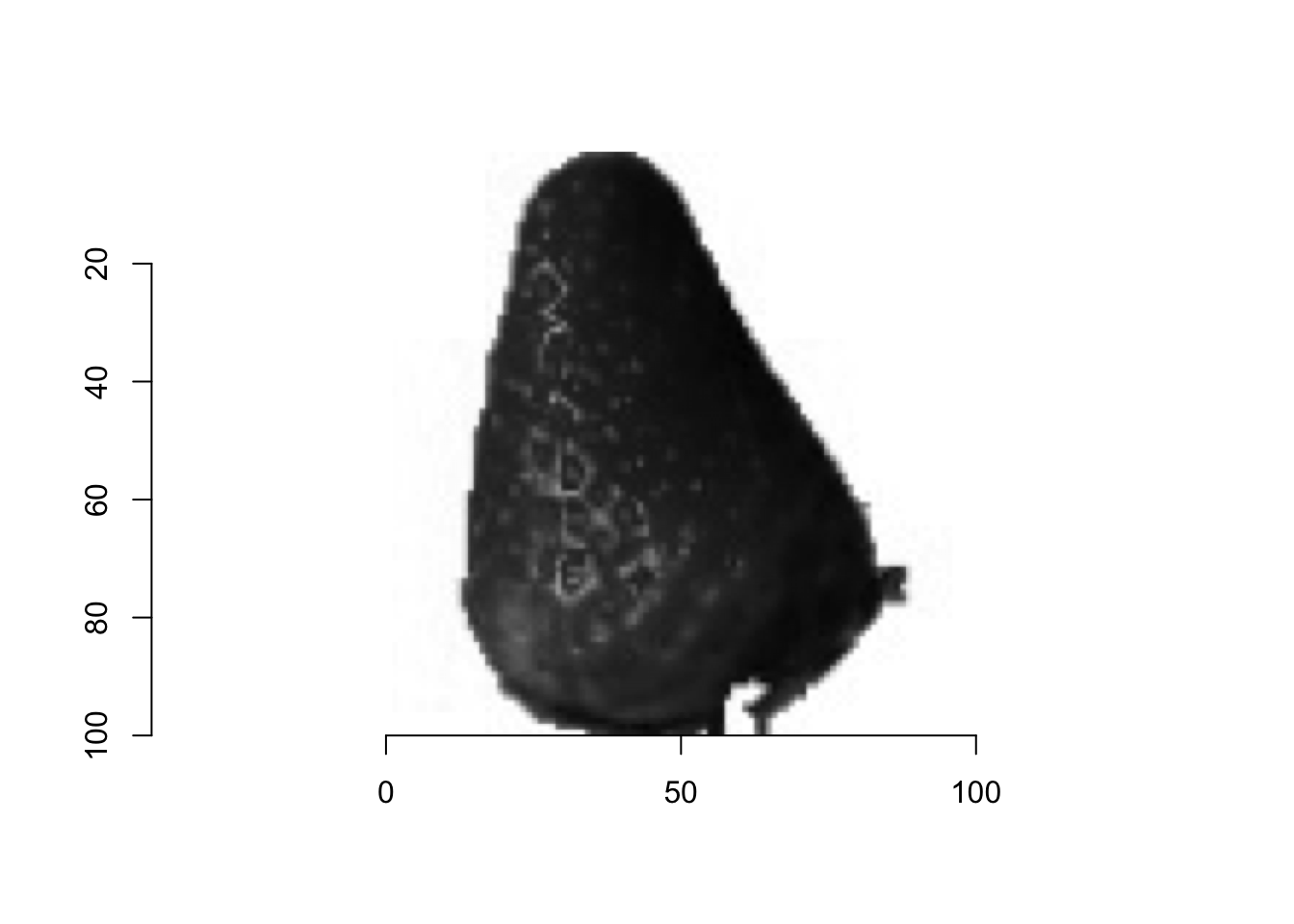

Our grey image has only one channel.

dim(im_grey)

## [1] 100 100   1   1

When we look at the actual matrix of pixel values (below, shown with a subset), we see that our values are not shown as raw values, but as scaled values between 0 and 1.

head(as.array(im_grey)[25:75, 25:75, 1, 1])

##           [,1]      [,2]      [,3]      [,4]      [,5]      [,6]      [,7]
## [1,] 0.2015294 0.1923529 0.2043529 0.2354902 0.2021961 0.2389804 0.2431373
## [2,] 0.2597647 0.2009804 0.2522745 0.3812941 0.2243137 0.2439608 0.2054902
## [3,] 0.2872941 0.2397255 0.3251765 0.5479608 0.3723922 0.2525882 0.2714510
## [4,] 0.2212549 0.2596078 0.5109020 0.2871765 0.5529412 0.2162745 0.5660000
## [5,] 0.2725882 0.3765882 0.2081569 0.1924314 0.3110196 0.3767843 0.6663922
## [6,] 0.4154118 0.2168627 0.2979216 0.1883922 0.1836471 0.5210196 0.4032549
##           [,8]      [,9]     [,10]     [,11]     [,12]     [,13]     [,14]
## [1,] 0.2787059 0.2401961 0.2547451 0.2709020 0.2475686 0.2474118 0.2561961
## [2,] 0.2407451 0.2520392 0.3678039 0.3932941 0.3570588 0.3727843 0.3171765
## [3,] 0.5352157 0.4680392 0.2788627 0.2087451 0.2096471 0.2569412 0.2856863
## [4,] 0.2663137 0.1769020 0.2441961 0.2172549 0.2004314 0.2517255 0.2801961
## [5,] 0.2470980 0.1892549 0.2169020 0.2211765 0.2041569 0.1972549 0.1933725
## [6,] 0.2209412 0.1961961 0.2166275 0.2123137 0.2503922 0.3057255 0.3998431
##          [,15]     [,16]     [,17]     [,18]     [,19]     [,20]     [,21]
## [1,] 0.2330980 0.2163529 0.2244706 0.2161961 0.1913725 0.2833725 0.1994902
## [2,] 0.2316863 0.2426275 0.2131765 0.2018431 0.2054902 0.2452157 0.2080392
## [3,] 0.2290196 0.2086667 0.2161176 0.2283922 0.2447059 0.2281176 0.2908627
## [4,] 0.2605882 0.2009412 0.2431765 0.4591765 0.6387843 0.3078824 0.2486275
## [5,] 0.1975686 0.2092549 0.2742745 0.4005882 0.3773333 0.2245490 0.2474902
## [6,] 0.3936471 0.1815294 0.1930980 0.2084706 0.5097647 0.3130196 0.2153333
##          [,22]     [,23]     [,24]     [,25]     [,26]     [,27]     [,28]
## [1,] 0.2122353 0.2283529 0.4250980 0.4372157 0.2789020 0.2011373 0.2278431
## [2,] 0.1925098 0.2745098 0.3172157 0.4366667 0.3427451 0.2161176 0.2557647
## [3,] 0.2150588 0.2788627 0.2544314 0.3665882 0.3292157 0.2121176 0.2092157
## [4,] 0.2119216 0.2029020 0.2005098 0.2485882 0.2550588 0.2402745 0.2172549
## [5,] 0.2466275 0.1983137 0.2108627 0.2305098 0.3066667 0.3615686 0.3726275
## [6,] 0.2040000 0.2472549 0.2114510 0.1891765 0.2429020 0.2867451 0.2863529
##          [,29]     [,30]     [,31]     [,32]     [,33]     [,34]     [,35]
## [1,] 0.2782353 0.3150980 0.3993725 0.3683922 0.3249804 0.3210588 0.3150588
## [2,] 0.2593333 0.2162353 0.2950588 0.4864706 0.4195294 0.4238039 0.3776863
## [3,] 0.2314510 0.2311765 0.2737255 0.3915686 0.3851765 0.4050588 0.4233725
## [4,] 0.2583922 0.2953333 0.3530196 0.3609412 0.4549020 0.4880000 0.4905882
## [5,] 0.4509804 0.5030980 0.4882745 0.4000784 0.4856863 0.6270196 0.5930196
## [6,] 0.2034118 0.1965882 0.2072157 0.2238824 0.2080392 0.2009804 0.5564314
##          [,36]     [,37]     [,38]     [,39]     [,40]     [,41]     [,42]
## [1,] 0.2461961 0.2352549 0.2726275 0.2752549 0.2603529 0.3112549 0.3981176
## [2,] 0.2441961 0.2152157 0.2407059 0.2647451 0.2650196 0.2767451 0.3592549
## [3,] 0.2318039 0.2348235 0.2612157 0.2647059 0.2647059 0.2958431 0.3112549
## [4,] 0.2630588 0.1901176 0.2414510 0.2483529 0.2601961 0.2713725 0.3139216
## [5,] 0.3403529 0.2250588 0.2315294 0.1954510 0.2704314 0.3076078 0.3111765
## [6,] 0.4018039 0.2904706 0.3806275 0.4549020 0.3765098 0.4278824 0.4952941
##          [,43]     [,44]     [,45]     [,46]     [,47]     [,48]     [,49]
## [1,] 0.3724706 0.3154902 0.3728627 0.3653333 0.3758824 0.4943922 0.4682353
## [2,] 0.3664706 0.3616863 0.3263922 0.2882745 0.2752157 0.2451373 0.3379608
## [3,] 0.3309804 0.2837647 0.2366275 0.2718039 0.2713725 0.2832549 0.2749020
## [4,] 0.3819216 0.3143137 0.2364706 0.2324314 0.2685098 0.2722745 0.2324706
## [5,] 0.2989804 0.2561176 0.2748627 0.3621961 0.5355686 0.4248235 0.6004314
## [6,] 0.4528627 0.3580392 0.2934118 0.4385098 0.2146275 0.2045882 0.2243922
##          [,50]     [,51]
## [1,] 0.3378039 0.2782353
## [2,] 0.2750980 0.3264314
## [3,] 0.2761961 0.3800000
## [4,] 0.3410980 0.5016863
## [5,] 0.6163922 0.6553333
## [6,] 0.2436471 0.2944706

The same applies to the color image, which if multiplied with 255 shows raw pixel values:

head(as.array(im)[25:75, 25:75, 1, 1]  * 255)

##      [,1] [,2] [,3] [,4] [,5] [,6] [,7] [,8] [,9] [,10] [,11] [,12] [,13]
## [1,]  138  142  150  161  151  155  153  161  158   156   155   144   143
## [2,]  159  139  147  183  152  159  135  127  144   174   177   164   162
## [3,]  170  140  143  200  172  150  139  184  185   148   139   133   134
## [4,]  142  138  189  130  204  119  200  114  114   148   152   141   140
## [5,]  138  172  139  133  145  146  220  122  132   149   153   140   127
## [6,]  170  141  184  155  127  190  162  129  147   150   144   148   155
##      [,14] [,15] [,16] [,17] [,18] [,19] [,20] [,21] [,22] [,23] [,24]
## [1,]   148   149   150   152   143   130   156   145   154   151   191
## [2,]   148   136   156   158   148   135   141   139   143   161   165
## [3,]   140   139   148   153   146   138   132   155   143   161   153
## [4,]   147   157   152   155   190   226   147   146   145   141   137
## [5,]   128   143   157   164   172   151   120   147   161   143   134
## [6,]   179   187   144   144   132   190   143   136   147   156   135
##      [,25] [,26] [,27] [,28] [,29] [,30] [,31] [,32] [,33] [,34] [,35]
## [1,]   190   157   141   139   144   152   176   167   150   149   159
## [2,]   177   170   153   162   152   136   155   197   167   164   162
## [3,]   162   165   148   147   146   140   144   163   147   151   170
## [4,]   143   149   147   138   143   148   157   149   165   172   185
## [5,]   150   165   172   169   185   197   193   169   187   216   206
## [6,]   143   149   152   147   125   123   127   137   133   120   198
##      [,36] [,37] [,38] [,39] [,40] [,41] [,42] [,43] [,44] [,45] [,46]
## [1,]   154   155   159   153   145   155   170   159   149   171   170
## [2,]   148   150   152   147   139   149   163   162   168   166   153
## [3,]   142   155   159   153   146   165   162   165   159   150   153
## [4,]   144   138   154   153   153   156   166   184   170   150   143
## [5,]   151   137   150   138   152   147   152   156   151   156   173
## [6,]   161   150   185   199   166   171   189   184   168   159   196
##      [,47] [,48] [,49] [,50] [,51]
## [1,]   170   200   200   174   165
## [2,]   143   135   167   160   176
## [3,]   146   148   150   150   174
## [4,]   148   149   139   159   190
## [5,]   215   191   237   233   229
## [6,]   136   133   141   143   148

Learning different levels of abstraction

These pixel arrays of our images are now the input to our CNN, which can now learn to recognize e.g. which fruit is on each image (a classification task). This is accomplished by learning different levels of abstraction of the images. In the first few hidden layers, the CNN usually detects general patterns, like edges; the deeper we go into the CNN, these learned abstractions become more specific, like textures, patterns and (parts of) objects.

MLPs versus CNNs

We could also train MLPs on our images but usually, they are not very good at this sort of task. So, what’s the magic behind CNNs, that makes them so much more powerful at detecting images and object?

The most important difference is that MLPs consider each pixel position as an independent features; it does not know neighboring pixels! That’s why MLPs will not be able to detect images where the objects have a different orientation, position, etc. Moreover, because we often deal with large images, the sheer number of trainable parameters in an MLP will quickly escalate, so that training such a network isn’t exactly efficient. CNNs consider groups of neighboring pixels. In the neural net these groups of neighboring pixels are only connected vertically with each other in the first CNN layers (until we collapse the information); this is called local connectivity. Because the CNN looks at pixels in context, it is able to learn patterns and objects and recognizes them even if they are in different positions on the image. These groups of neighboring pixels are scanned with a sliding window, which runs across the entire image from the top left corner to the bottom right corner. The size of the sliding window can vary, often we find e.g. 3x3 or 5x5 pixel windows.

In MLPs, weights are learned, e.g. with gradient descent and backpropagation. CNNs (convolutional layers to be specific) learn so called filters or kernels (sometimes also called filter kernels). The number of trainable parameters can be much lower in CNNs than in a MLP!

By the way, CNNs can not only be used to classify images, they can also be used for other tasks, like text classification!

Learning filter kernels

A filter is a matrix with the same dimension as our sliding window, e.g. 3x3. At each position of our sliding window, a mathematical operation is performed, the so called convolution. During convolution, each pixel value in our window is multiplied with the value at the respective position in the filter matrix and the sum of all multiplications is calculated. This result is called the dot product. Depending on what values the filter contains at which position, the original image will be transformed in a certain way, e.g. sharpen, blur or make edges stand out. You can find great visualizations on setosa.io.

To be precise, filters are collections of kernels so that, if we work with color images, we have 3 channels. The 3 dimensions from the channels will all get one kernel, which together create the filter. Each filter will only calculate one output value, the dot product mentioned earlier. The learning part of CNNs comes into play with these filters. Similar to learning weights in a MLP, CNNs will learn the most optimal filters for recognizing specific objects and patterns. But a CNN doesn’t only learn one filter, it learns multiple filters. In fact, it even learns multiple filters in each layer! Every filter learns a specific pattern, or feature. That’s why these collections of parallel filters are the so called stacks of feature maps or activation maps. We can visualize these activation maps to help us understand what the CNN learn along the way, but this is a topic for another lesson.

Padding and step size

Two important hyperparameters of CNNs are padding and step size. Padding means the (optional) adding of “fake” pixel values to the borders of the images. This is done to scan all pixels the same number of times with the sliding window (otherwise the border pixels would get covered less frequently than pixels in the center of the image) and to keep the the size of the image the same between layers (otherwise the output image would be smaller than the input image). There are different options for padding, with “same” the border pixels will be duplicated or you could pad with zeros. Now our sliding window can start “sliding”. The step size determines how far the window will proceed between convolutions. Often we find a step size of 1, where the sliding window will advance only 1 pixel to the right and to the bottom while scanning the image. If we increase the step size, we would need to do fewer calculations and our model would train faster. Also, we would reduce the output image size; in modern implementations, this is explicitly done for that purpose, instead of using pooling layers.

Pooling

As you can probably guess from the previous sentence, pooling layers are used to reduce the size of images in a CNN and to compress the information down to a smaller scale. Pooling is applied to every feature map and helps to extract broader and more general patterns that are more robust to small changes in the input. Common CNN architectures combine one or two convolutional layers with one pooling layer in one block. Several of such blocks are then put in a row to form the core of a basic CNN. Several advancements to this basic architecture exist nowadays, like Inception/Xception, ResNets, etc. but I will focus on the basics here (an advanced chapter will be added to the course in the future).

Pooling layers also work with sliding windows; they can but don’t have to have the same dimension as the sliding window from the convolutional layer. Also, sliding windows for pooling normally don’t overlap and every pixel is only considered once. There are several options for how to pool:

• max pooling will keep only the biggest value of each window
• average pooling will build the average from each window
• sum pooling will build the sum of each window

Dense layers calculate the output of the CNN

After our desired number of convolution + pooling blocks, there will usually be a few dense (or fully connected) layers before the final dense layer that calculates the output. These dense layers are nothing else than a simple MLP that learns the classification or regression task, while you can think of the preceding convolutions as the means to extract the relevant features for this simple MLP.

Just like in a MLP, we use activation functions, like rectified linear units in our CNN; here, they are used with convolutional layers and dense layers. Because pooling only condenses information, we don’t need to normalize the output there.

You can find the R version of the Python code, which we provide for this course in this blog article.

Video:

Slides:

sessionInfo()

## R version 3.5.1 (2018-07-02)
## Platform: x86_64-apple-darwin15.6.0 (64-bit)
## Running under: macOS  10.14.2
## 
## Matrix products: default
## BLAS: /Library/Frameworks/R.framework/Versions/3.5/Resources/lib/libRblas.0.dylib
## LAPACK: /Library/Frameworks/R.framework/Versions/3.5/Resources/lib/libRlapack.dylib
## 
## locale:
## [1] en_US.UTF-8/en_US.UTF-8/en_US.UTF-8/C/en_US.UTF-8/en_US.UTF-8
## 
## attached base packages:
## [1] stats     graphics  grDevices utils     datasets  methods   base     
## 
## other attached packages:
## [1] imager_0.41.1 magrittr_1.5 
## 
## loaded via a namespace (and not attached):
##  [1] Rcpp_1.0.0       bookdown_0.9     png_0.1-7        digest_0.6.18   
##  [5] tiff_0.1-5       plyr_1.8.4       evaluate_0.12    blogdown_0.9    
##  [9] rlang_0.3.0.1    stringi_1.2.4    bmp_0.3          rmarkdown_1.11  
## [13] tools_3.5.1      stringr_1.3.1    purrr_0.2.5      igraph_1.2.2    
## [17] jpeg_0.1-8       xfun_0.4         yaml_2.2.0       compiler_3.5.1  
## [21] pkgconfig_2.0.2  htmltools_0.3.6  readbitmap_0.1.5 knitr_1.21