
The Good, the Bad and the Ugly: how (not) to visualize data
Below you’ll find the complete code used to create the ggplot2 graphs in my talk The Good, the Bad and the Ugly: how (not) to visualize data at this year’s data2day conference. You can find the German slides here:
You can also find a German blog article accompanying my talk on codecentric’s blog.
If you have questions or would like to talk about this article (or something else data-related), you can now book 15-minute timeslots with me (it’s free - one slot available per weekday):

If you have been enjoying my content and would like to help me be able to create more, please consider sending me a donation at . Thank you! :-)
library(tidyverse)

library(ggExtra)
library(ragg)
library(ggalluvial)
library(treemapify)
library(ggalt)

library(palmerpenguins)
Dataset
head(penguins)## # A tibble: 6 x 8
## species island bill_length_mm bill_depth_mm flipper_length_… body_mass_g sex
## <fct> <fct> <dbl> <dbl> <int> <int> <fct>
## 1 Adelie Torge… 39.1 18.7 181 3750 male
## 2 Adelie Torge… 39.5 17.4 186 3800 fema…
## 3 Adelie Torge… 40.3 18 195 3250 fema…
## 4 Adelie Torge… NA NA NA NA <NA>
## 5 Adelie Torge… 36.7 19.3 193 3450 fema…
## 6 Adelie Torge… 39.3 20.6 190 3650 male
## # … with 1 more variable: year <int>#head(penguins_raw)Colors
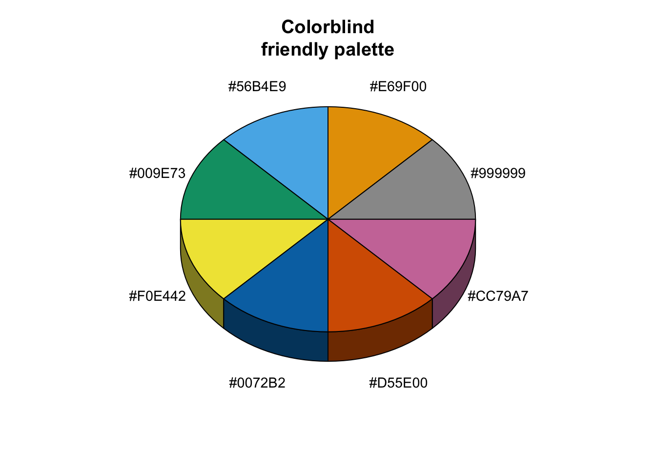
# The palette with grey:
cbp1 <- c("#999999", "#E69F00", "#56B4E9", "#009E73",
          "#F0E442", "#0072B2", "#D55E00", "#CC79A7")

# The palette with black:
cbp2 <- c("#000000", "#E69F00", "#56B4E9", "#009E73",
          "#F0E442", "#0072B2", "#D55E00", "#CC79A7")

library(plotrix)
sliceValues <- rep(10, 8) # each slice value=10 for proportionate slices
(
  p <- pie3D(sliceValues,
      explode=0,
      theta = 1.2,
      col = cbp1,
      labels = cbp1,
      labelcex = 0.9,
      shade = 0.6,
      main = "Colorblind\nfriendly palette")
)
## [1] 0.3926991 1.1780972 1.9634954 2.7488936 3.5342917 4.3196899 5.1050881
## [8] 5.8904862
ggplot <- function(...) ggplot2::ggplot(...) +
scale_color_manual(values = cbp1) +
scale_fill_manual(values = cbp1) + # note: needs to be overridden when using continuous color scales
theme_bw()Main diagram types
https://rstudio.com/wp-content/uploads/2015/03/ggplot2-cheatsheet.pdf
Pointcharts
penguins %>%
    remove_missing() %>%
    ggplot(aes(x = bill_length_mm, y = flipper_length_mm)) +
    geom_jitter(alpha = 0.5) +
    facet_wrap(vars(species), ncol = 3) +
    scale_x_reverse() +
    scale_y_reverse() +
    labs(x = "Bill length (mm)",
         y = "Flipper length (mm)",
         size = "body mass (g)",
        title = "Scatterplot",
        subtitle = "Penguins bill v. flipper length by species",
        caption = "Source: https://github.com/allisonhorst/palmerpenguins")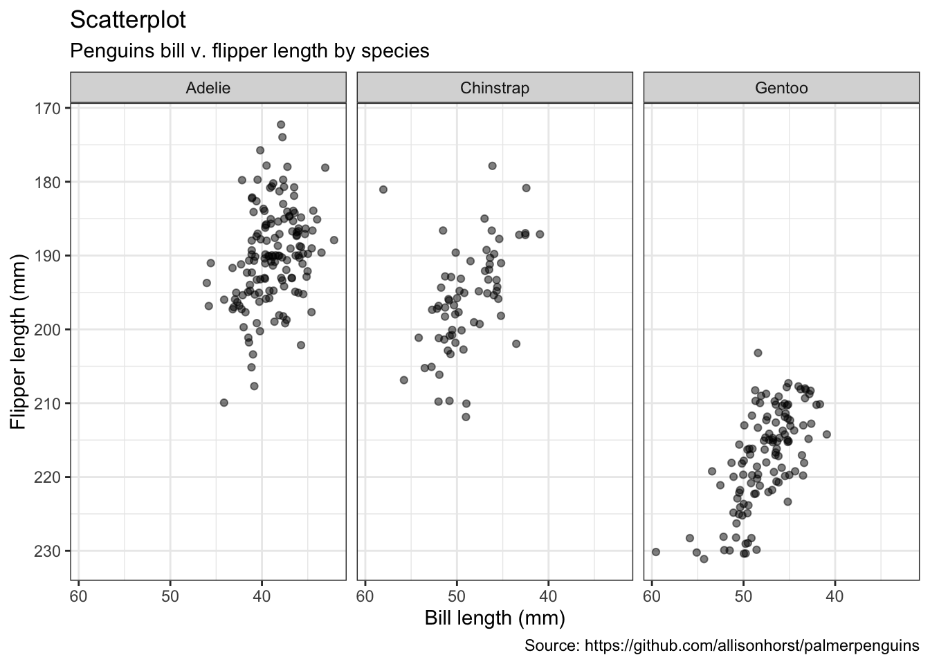
penguins %>%
    remove_missing() %>%
    ggplot(aes(x = bill_length_mm, y = flipper_length_mm,
              color = species, shape = species)) +
    geom_point(alpha = 0.7) +
    labs(x = "Bill length (mm)",
         y = "Flipper length (mm)",
        title = "Scatterplot",
        subtitle = "Penguins bill v. flipper length by species",
        caption = "Source: https://github.com/allisonhorst/palmerpenguins")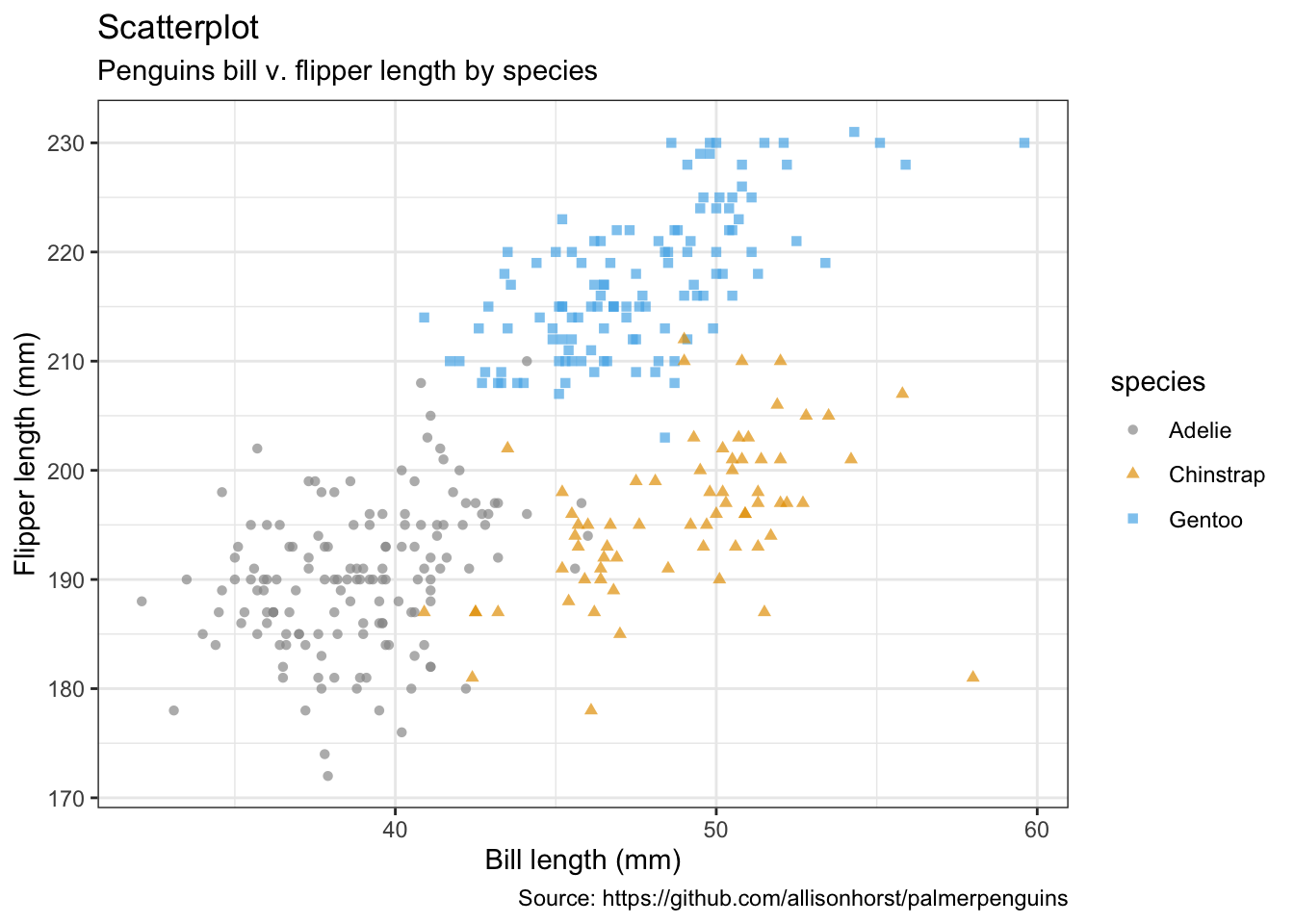
- Jitter with smoothing line
penguins %>%
    remove_missing() %>%
    ggplot(aes(x = bill_length_mm, y = flipper_length_mm,
              color = species, shape = species)) +
    geom_jitter(alpha = 0.5) +
    geom_smooth(method = "loess", se = TRUE) +
    facet_wrap(vars(species), nrow = 3) +
    labs(x = "Bill length (mm)",
         y = "Flipper length (mm)",
        title = "Scatterplot with smoothing line",
        subtitle = "Penguins bill v. flipper length by species with loess smoothing line",
        caption = "Source: https://github.com/allisonhorst/palmerpenguins")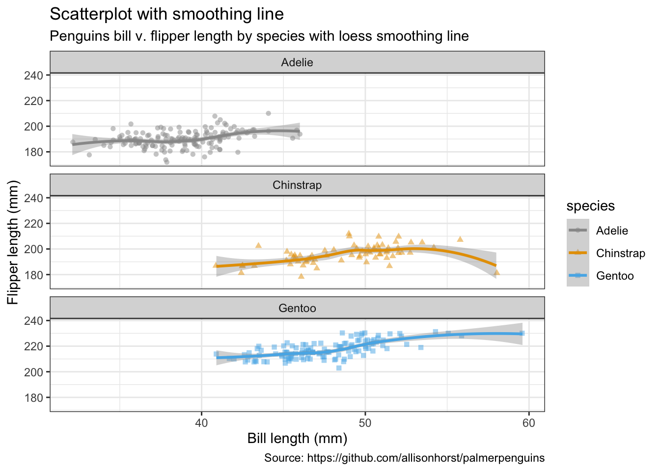
penguins %>%
  remove_missing() %>%
  filter(species == "Adelie") %>%
  ggplot(aes(x = bill_length_mm, y = flipper_length_mm)) +
  geom_point(alpha = 0.5) +
  geom_smooth(method = "loess", se = TRUE) +
    labs(x = "Bill length (mm)",
         y = "Flipper length (mm)",
        title = "Scatterplot with smoothing line",
        subtitle = "Penguins bill v. flipper length by species with\nloess smoothing line, histogram & density distribution",
        caption = "Source: https://github.com/allisonhorst/palmerpenguins")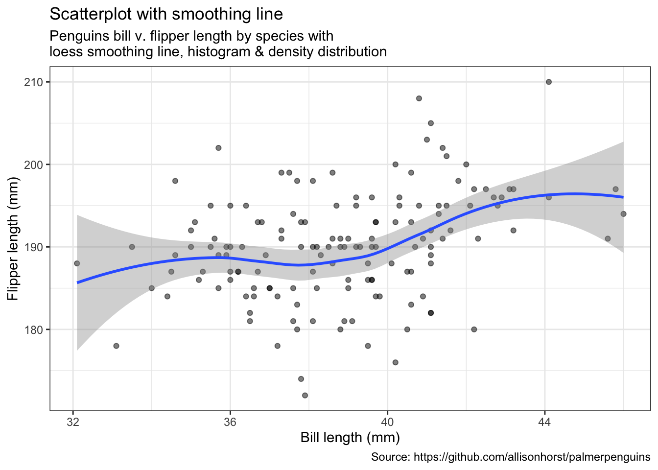
#(ggMarginal(p, type = "densigram", fill = "transparent"))Bubblecharts
penguins %>%
    remove_missing() %>%
    ggplot(aes(x = bill_length_mm, y = flipper_length_mm,
              color = species, shape = species, size = body_mass_g)) +
    geom_point(alpha = 0.5) +
    labs(x = "Bill length (mm)",
         y = "Flipper length (mm)",
        title = "Bubble plot",
        size = "body mass (g)",
        subtitle = "Penguins bill v. flipper length by species;\nsize indicates body mass in grams",
        caption = "Source: https://github.com/allisonhorst/palmerpenguins")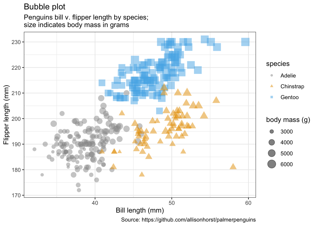
Linecharts
penguins %>%
    remove_missing() %>%
    filter(species == "Adelie") %>%
    ggplot(aes(x = bill_length_mm, y = flipper_length_mm,
               color = sex)) +
    geom_line() +
    geom_point() +
    labs(x = "Bill length (mm)",
         y = "Flipper length (mm)",
        title = "Line plot",
        subtitle = "Penguins bill v. flipper length by species and sex",
        caption = "Source: https://github.com/allisonhorst/palmerpenguins")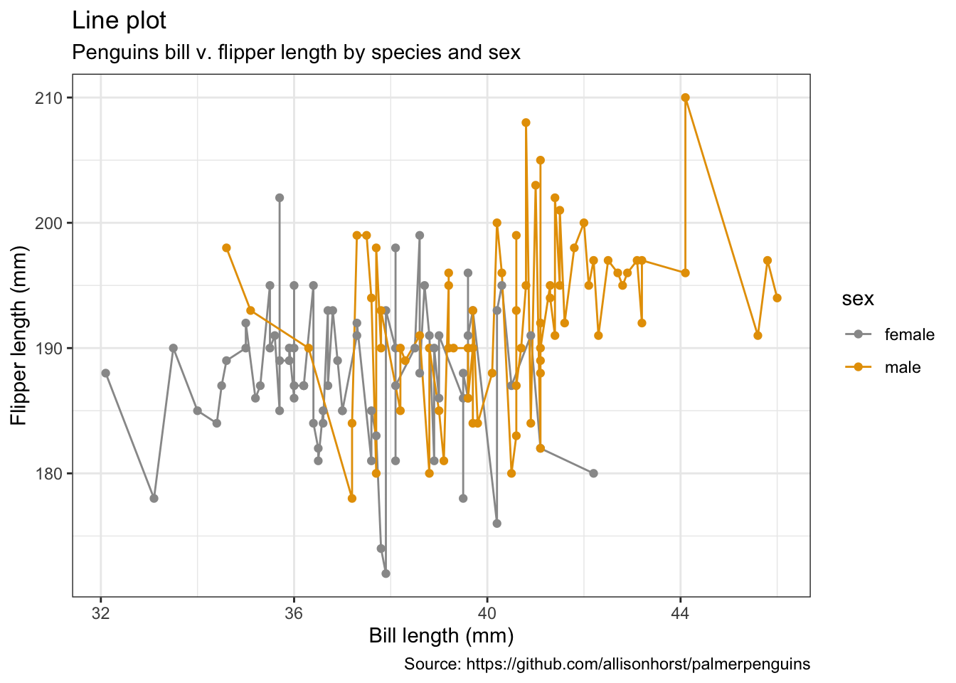
Correlation plots / heatmaps
mat <- penguins %>%
  remove_missing() %>%
  select(bill_depth_mm, bill_length_mm, body_mass_g, flipper_length_mm)

cormat <- round(cor(mat), 2)
cormat[upper.tri(cormat)] <- NA

cormat <- cormat %>%
  as_data_frame() %>%
  mutate(x = colnames(mat)) %>%
  gather(key = "y", value = "value", bill_depth_mm:flipper_length_mm)

cormat %>%
    remove_missing() %>%
    arrange(x, y) %>%
    ggplot(aes(x = x, y = y, fill = value)) +
    geom_tile() +
    scale_fill_gradient2(low = "blue", high = "red", mid = "white",
     midpoint = 0, limit = c(-1,1), space = "Lab",
     name = "Pearson\nCorrelation") +
    theme(axis.text.x = element_text(angle = 45, vjust = 1, hjust = 1)) +
    coord_fixed() +
      labs(x = "",
           y = "",
          title = "Correlation heatmap",
          subtitle = "Correlation btw. penguins' traits",
          caption = "Source: https://github.com/allisonhorst/palmerpenguins")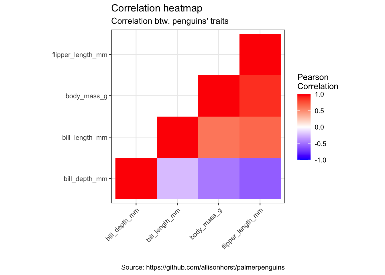
Barcharts
- per default: counts
penguins %>%
    remove_missing() %>%
    ggplot(aes(x = species,
               fill = sex)) +
    geom_bar() +
      labs(x = "Species",
           y = "Counts",
          title = "Barchart",
          subtitle = "Counts of male & female penguins per species in study",
          caption = "Source: https://github.com/allisonhorst/palmerpenguins")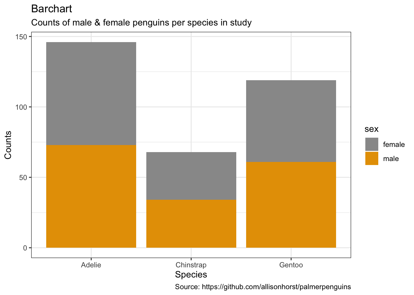
penguins %>%
    remove_missing() %>%
    ggplot(aes(x = species,
               fill = sex)) +
    geom_bar(position = 'dodge') +
      labs(x = "Species",
           y = "Counts",
          title = "Barchart",
          subtitle = "Counts of male & female penguins per species in study",
          caption = "Source: https://github.com/allisonhorst/palmerpenguins")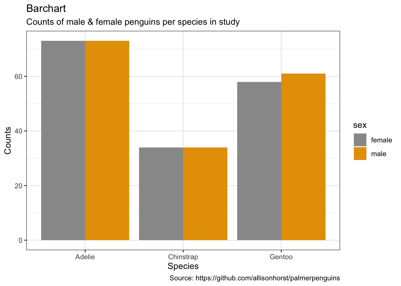
- alternative: set y-values
penguins %>%
    remove_missing() %>%
    group_by(species, sex) %>%
    summarise(mean_bmg = mean(body_mass_g),
              sd_bmg = sd(body_mass_g)) %>%
    ggplot(aes(x = species, y = mean_bmg,
               fill = sex)) +
    geom_bar(stat = "identity", position = "dodge") +
    geom_errorbar(aes(ymin = mean_bmg - sd_bmg,
                      ymax = mean_bmg + sd_bmg),
                  width = 0.2,
                 position = position_dodge(0.9)) +
      labs(x = "Species",
           y = "Mean body mass (in g)",
          title = "Barchart",
          subtitle = "Mean body mass of male & female penguins per species\nwith standard deviation",
          caption = "Source: https://github.com/allisonhorst/palmerpenguins")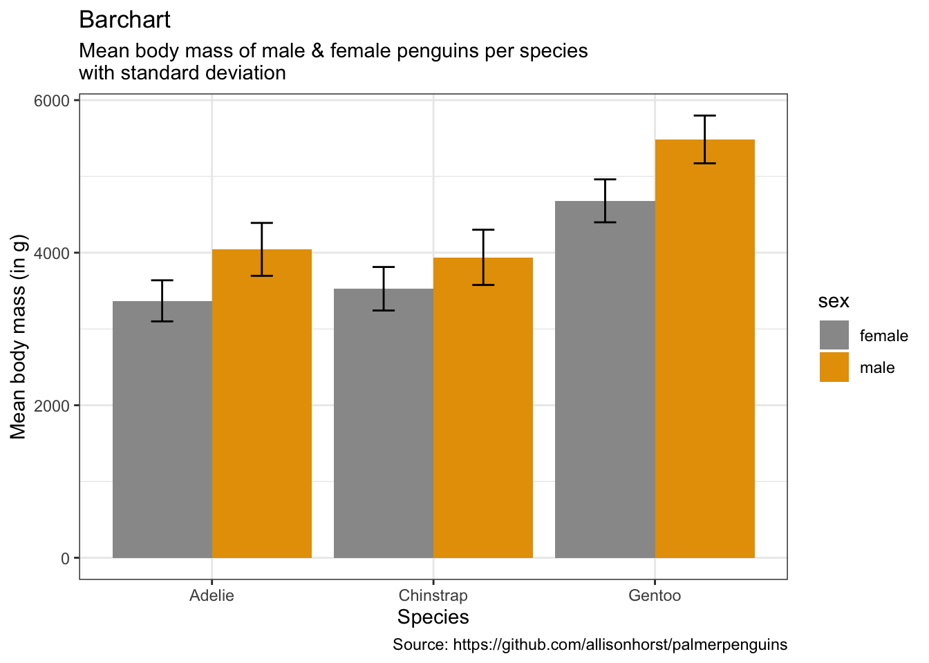
Boxplots
penguins %>%
    remove_missing() %>%
    ggplot(aes(x = species, y = body_mass_g,
               fill = sex)) +
    geom_boxplot() +
      labs(x = "Species",
           y = "Body mass (in g)",
          title = "Boxplot",
          subtitle = "Body mass of three penguin species per sex",
          caption = "Source: https://github.com/allisonhorst/palmerpenguins")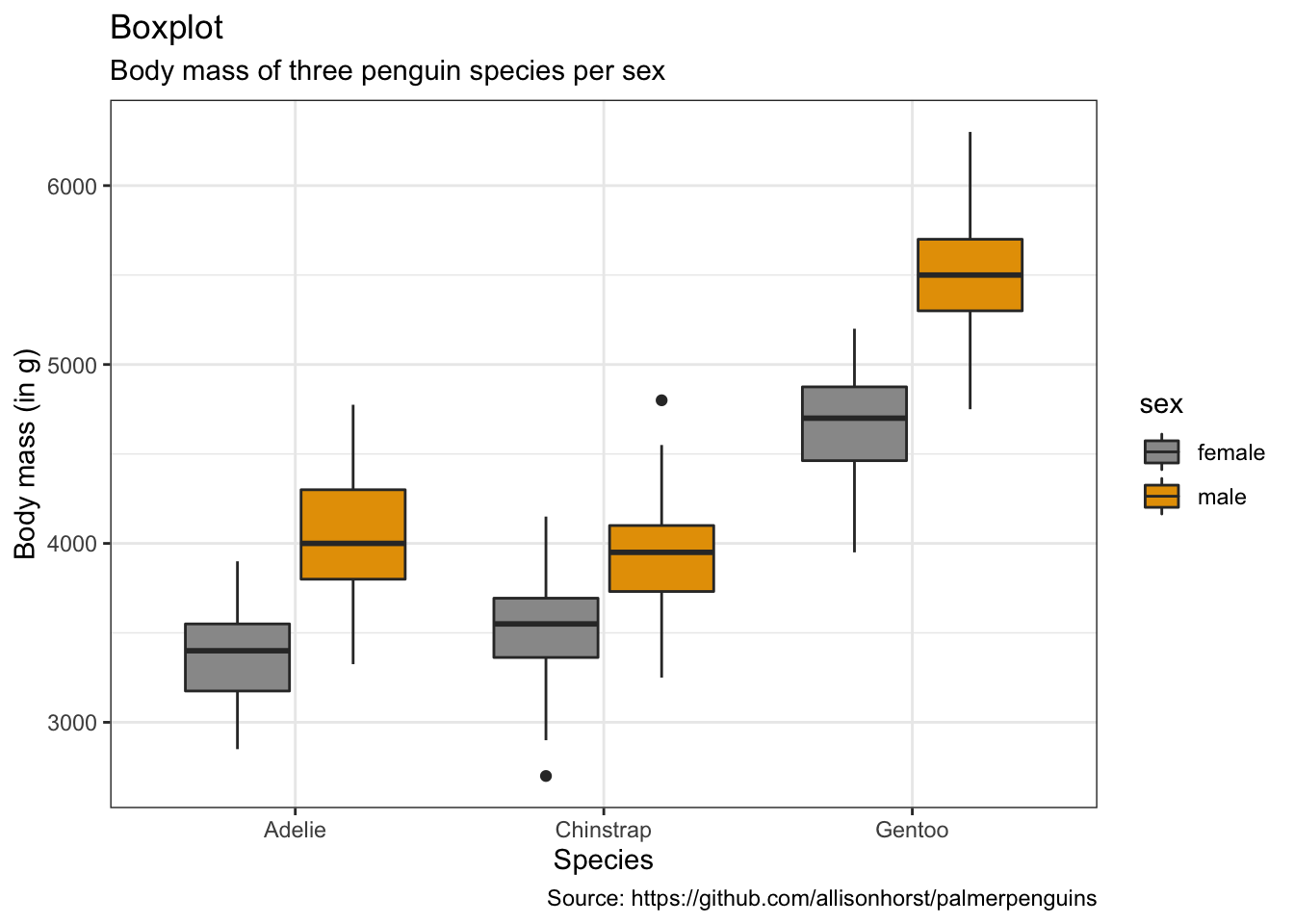
- with points
penguins %>%
    remove_missing() %>%
    ggplot(aes(x = species, y = body_mass_g,
               fill = sex, color = sex)) +
    geom_boxplot(alpha = 0.5, notch = TRUE) +
    geom_jitter(alpha = 0.5, position=position_jitter(0.3)) +
      labs(x = "Species",
           y = "Body mass (in g)",
          title = "Boxplot with points (dotplot)",
          subtitle = "Body mass of three penguin species per sex",
          caption = "Source: https://github.com/allisonhorst/palmerpenguins")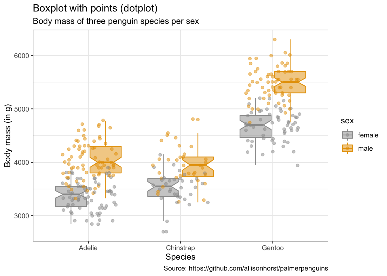
Violinplots
penguins %>%
    remove_missing() %>%
    ggplot(aes(x = species, y = body_mass_g,
               fill = sex)) +
    geom_violin(scale = "area") +
      labs(x = "Species",
           y = "Body mass (in g)",
          title = "Violinplot",
          subtitle = "Body mass of three penguin species per sex",
          caption = "Source: https://github.com/allisonhorst/palmerpenguins")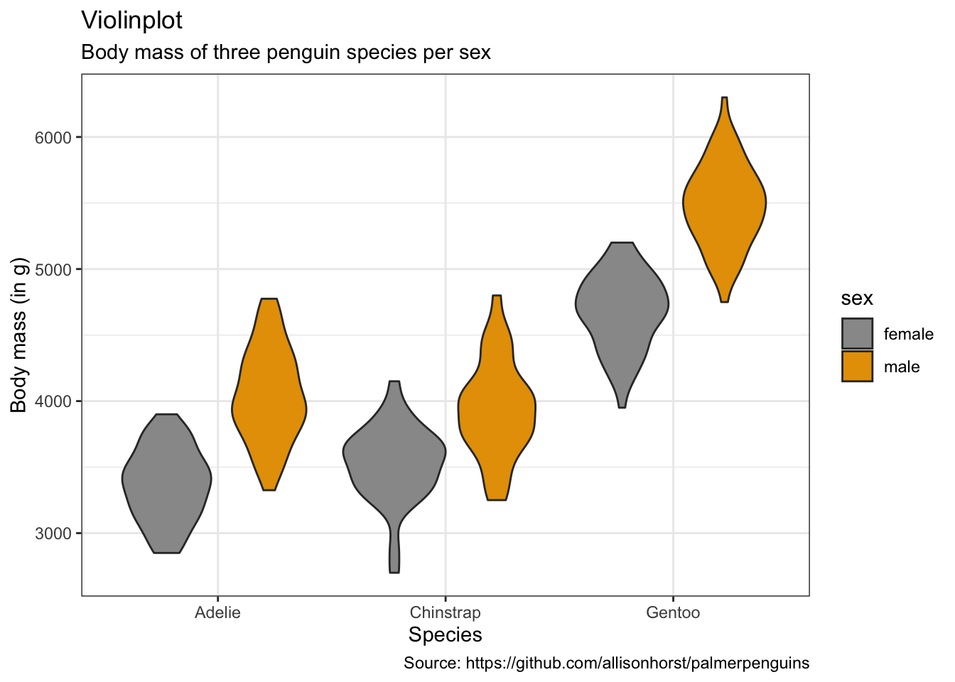
- with dots (sina-plots)
penguins %>%
    remove_missing() %>%
    ggplot(aes(x = species, y = body_mass_g,
               fill = sex, color = sex)) +
    geom_dotplot(method = "dotdensity", alpha = 0.7,
                 binaxis = 'y', stackdir = 'center',
                 position = position_dodge(1)) +
      labs(x = "Species",
           y = "Body mass (in g)",
          title = "Violinplot with points (dotplot)",
          subtitle = "Body mass of three penguin species per sex",
          caption = "Source: https://github.com/allisonhorst/palmerpenguins")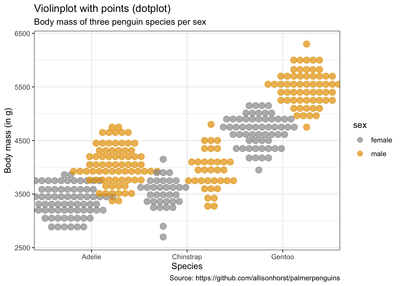
Piecharts
penguins %>%
    remove_missing() %>%
    group_by(species, sex) %>%
    summarise(n = n()) %>%
    mutate(freq = n / sum(n),
           percentage = freq * 100) %>%
    ggplot(aes(x = "", y = percentage,
               fill = sex)) +
    facet_wrap(vars(species), nrow = 1) +
    geom_bar(stat = "identity", alpha = 0.8) +
    coord_polar("y", start = 0) +
      labs(x = "",
           y = "Percentage",
          title = "Piechart",
          subtitle = "Percentage of male v. female penguins per species in study",
          caption = "Source: https://github.com/allisonhorst/palmerpenguins")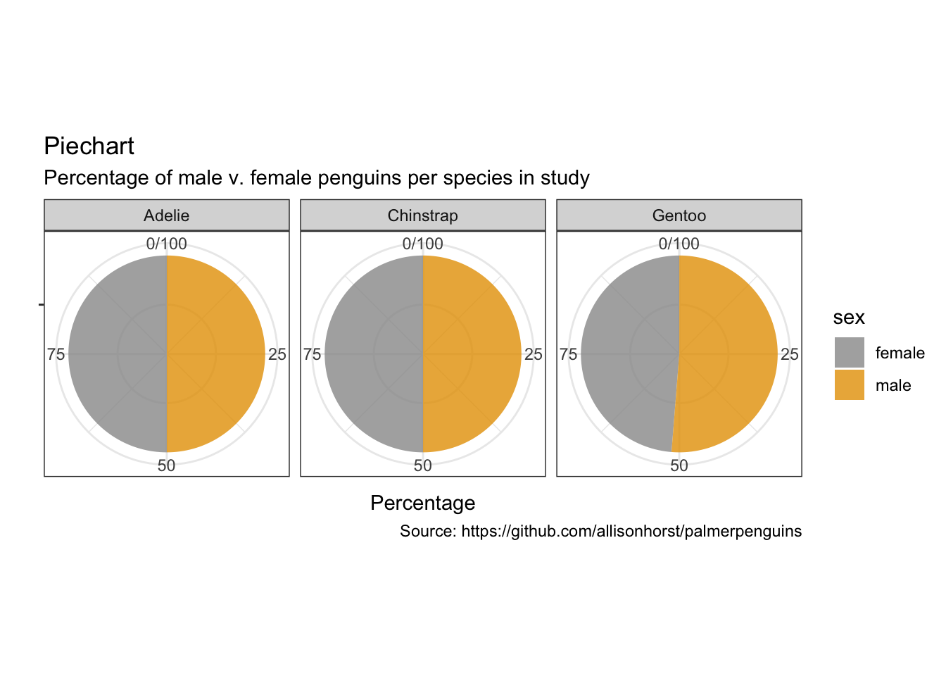
Alluvial charts
as.data.frame(UCBAdmissions) %>%
    ggplot(aes(y = Freq, axis1 = Gender, axis2 = Dept)) +
    geom_alluvium(aes(fill = Admit), width = 1/12) +
    geom_stratum(width = 1/12, fill = "black", color = "grey") +
    geom_label(stat = "stratum", aes(label = after_stat(stratum))) +
    scale_x_discrete(limits = c("Gender", "Dept"), expand = c(.05, .05)) +
      labs(x = "",
           y = "Frequency",
          title = "Alluvial chart",
          subtitle = "UC Berkeley admissions and rejections, by sex and department",
          caption = "Source: Bickel et al. (1975)\nSex bias in graduate admissions: Data from Berkeley. Science, 187, 398–403.")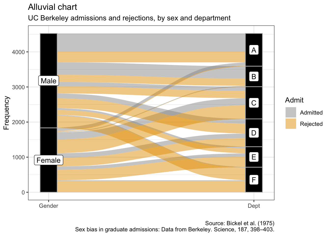
Treemaps
as.data.frame(UCBAdmissions) %>%
    group_by(Admit, Gender) %>%
    summarise(sum_freq = sum(Freq)) %>%
    ggplot(aes(area = sum_freq, fill = sum_freq, label = Gender,
               subgroup = Admit)) +
    geom_treemap() +
    geom_treemap_subgroup_border() +
    geom_treemap_subgroup_text(place = "centre", grow = T, alpha = 0.5, colour =
                             "black", fontface = "italic", min.size = 0) +
    geom_treemap_text(colour = "white", place = "centre", reflow = T) +
    scale_fill_gradient2(low = "#999999", high = "#E69F00", mid = "white", midpoint = 1000, space = "Lab",
     name = "Sum of\nfrequencies") +
      labs(x = "",
           y = "",
          title = "Treemap",
          subtitle = "UC Berkeley admissions and rejections by sex",
          caption = "Source: Bickel et al. (1975)\nSex bias in graduate admissions: Data from Berkeley. Science, 187, 398–403.")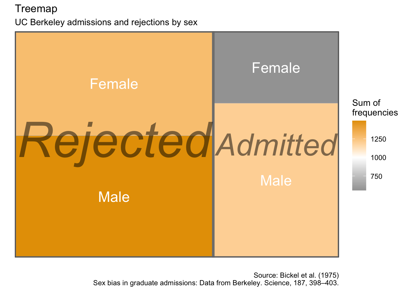
Dumbbell plots
penguins %>%
    remove_missing() %>%
    group_by(year, species, sex) %>%
    summarise(mean_bmg = mean(body_mass_g)) %>%
    mutate(species_sex = paste(species, sex, sep = "_"),
         year = paste0("year_", year)) %>%
    spread(year, mean_bmg) %>%
    ggplot(aes(x = year_2007, xend = year_2009,
               y = reorder(species_sex, year_2009))) +
    geom_dumbbell(color = "#999999",
                      size_x = 3,
                      size_xend = 3,
                      #Note: there is no US:'color' for UK:'colour'
                      # in geom_dumbbel unlike standard geoms in ggplot()
                      colour_x = "#999999",
                      colour_xend = "#E69F00") +
      labs(x = "Body mass (g)",
           y = "Species & sex",
          title = "Dumbbell plot",
          subtitle = "Penguin's change in body mass from 2007 to 2009",
          caption = "Source: https://github.com/allisonhorst/palmerpenguins")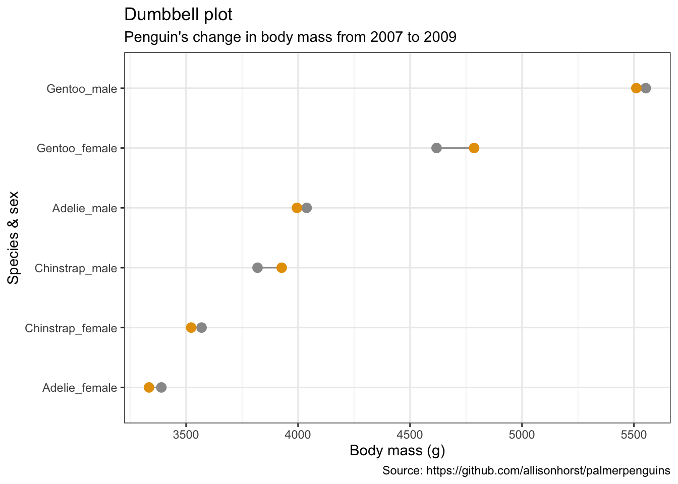
Slope charts
penguins %>%
    remove_missing() %>%
    group_by(year, species, sex) %>%
    summarise(mean_bmg = mean(body_mass_g)) %>%
    ggplot(aes(x = year, y = mean_bmg, group = sex,
               color = sex)) +
    facet_wrap(vars(species), nrow = 3) +
    geom_line(alpha = 0.6, size = 2) +
    geom_point(alpha = 1, size = 3) +
    scale_x_continuous(breaks=c(2007, 2008, 2009)) +
      labs(x = "Year",
           y = "Body mass (g)",
           color = "Sex",
          title = "Slope chart",
          subtitle = "Penguin's change in body mass from 2007 to 2009",
          caption = "Source: https://github.com/allisonhorst/palmerpenguins")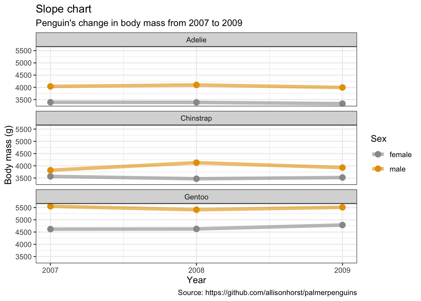
Stacked area charts
penguins %>%
    remove_missing() %>%
    group_by(year, species, sex) %>%
    summarise(mean_bmg = mean(body_mass_g)) %>%
    ggplot(aes(x = year, y = mean_bmg, fill = sex)) +
    facet_wrap(vars(species), nrow = 3) +
    geom_area(alpha = 0.6, size=.5, color = "white") +
    scale_x_continuous(breaks=c(2007, 2008, 2009)) +
      labs(x = "Year",
           y = "Mean body mass (g)",
           color = "Sex",
          title = "Stacked area chart",
          subtitle = "Penguin's change in body mass from 2007 to 2009",
          caption = "Source: https://github.com/allisonhorst/palmerpenguins")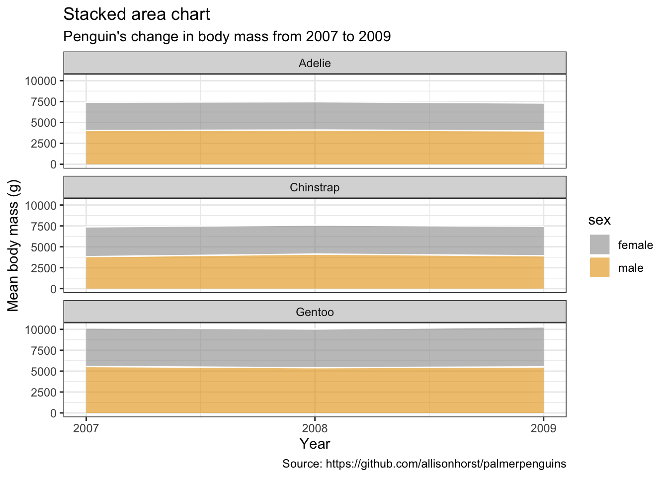
Lolliplot chart
penguins %>%
    remove_missing() %>%
    group_by(year, species, sex) %>%
    summarise(mean_bmg = mean(body_mass_g)) %>%
    mutate(species_sex = paste(species, sex, sep = "_"),
         year = paste0("year_", year)) %>%
    spread(year, mean_bmg) %>%
    ggplot() +
    geom_segment(aes(x = reorder(species_sex, -year_2009), xend = reorder(species_sex, -year_2009),
                   y = 0, yend = year_2009),
                 color = "#999999", size = 1) +
    geom_point(aes(x = reorder(species_sex, -year_2009), y = year_2009),
               size = 4, color = "#E69F00") +
    coord_flip() +
      labs(x = "Species & sex",
           y = "Body mass (g)",
          title = "Lollipop chart",
          subtitle = "Penguin's body mass in 2009",
          caption = "Source: https://github.com/allisonhorst/palmerpenguins")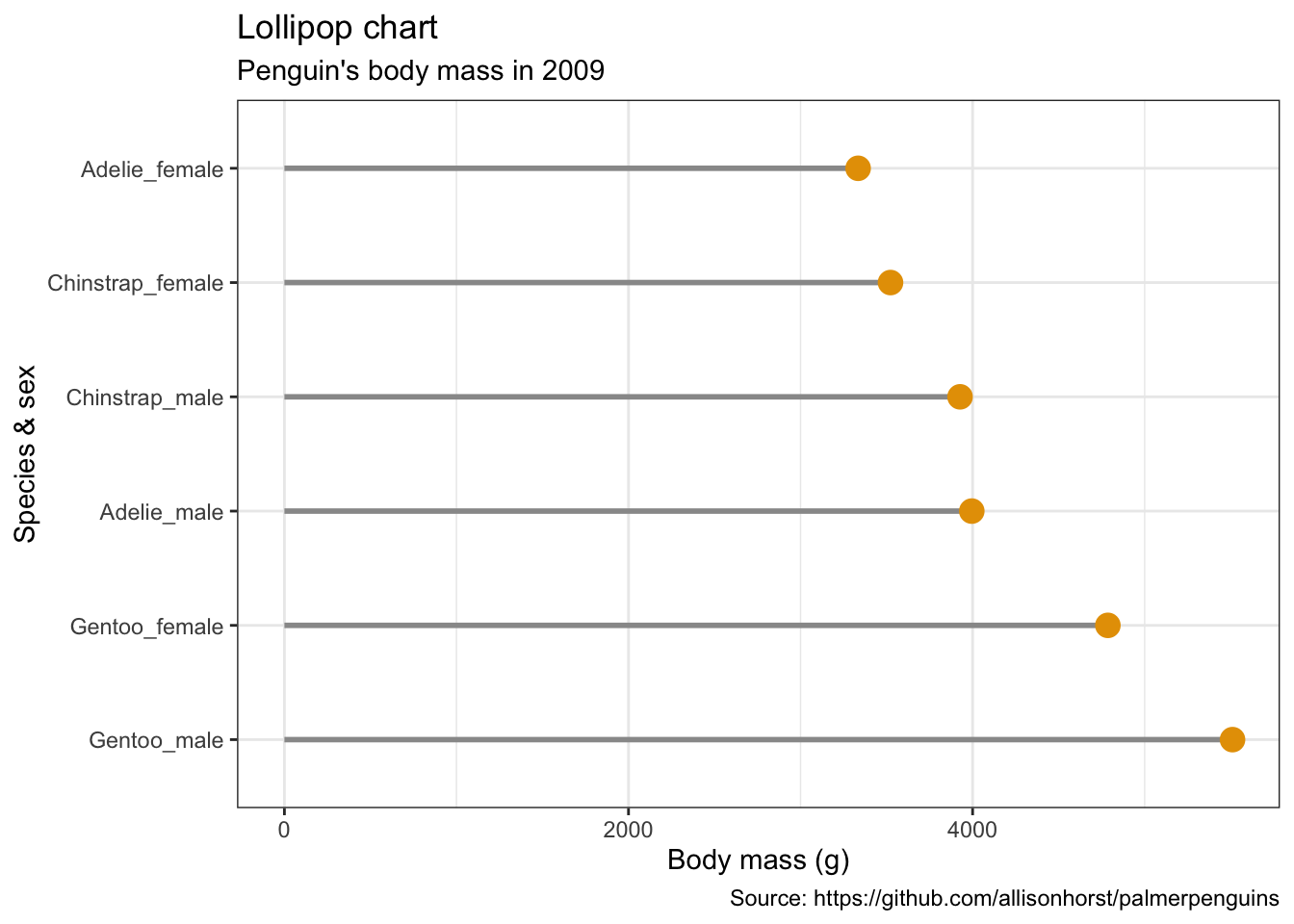
Dendrograms
library(ggdendro)
library(dendextend)
penguins_hist <- penguins %>%
filter(sex == "male") %>%
select(species, bill_length_mm, bill_depth_mm, flipper_length_mm, body_mass_g) %>%
group_by(species) %>%
sample_n(10) %>%
as.data.frame()
rownames(penguins_hist) <- paste(penguins_hist$species, seq_len(nrow(penguins_hist)), sep = "_")
penguins_hist <- penguins_hist %>%
select(-species) %>%
remove_missing()#hc <- hclust(dist(penguins_hist, method = "euclidean"), method = "ward.D2")
#ggdendrogram(hc)
# Create a dendrogram and plot it
penguins_hist %>%
scale %>%
dist(method = "euclidean") %>%
hclust(method = "ward.D2") %>%
as.dendrogram## 'dendrogram' with 2 branches and 30 members total, at height 11.94105Waterfall charts
library(waterfall)jaquith %>%
arrange(score) %>%
add_row(factor = "Total", score = sum(jaquith$score)) %>%
mutate(factor = factor(factor, levels = factor),
id = seq_along(score)) %>%
mutate(end = cumsum(score),
start = c(0, end[-length(end)]),
start = c(start[-length(start)], 0),
end = c(end[-length(end)], score[length(score)]),
gr_col = ifelse(factor == "Total", "Total", "Part")) %>%
ggplot(aes(x = factor, fill = gr_col)) +
geom_rect(aes(x = factor,
xmin = id - 0.45, xmax = id + 0.45,
ymin = end, ymax = start)) +
theme(axis.text.x = element_text(angle = 60, vjust = 1, hjust = 1),
legend.position = "none") +
labs(x = "",
y = "Amount",
title = "Waterfall chart",
subtitle = "Sample business-adjusted risk from Security Metrics",
caption = "Andrew Jaquith, Security Metrics: Replacing Fear, Uncertainty, and Doubt\n(Boston: Addison-Wesley Professional, 2007), 170-171.")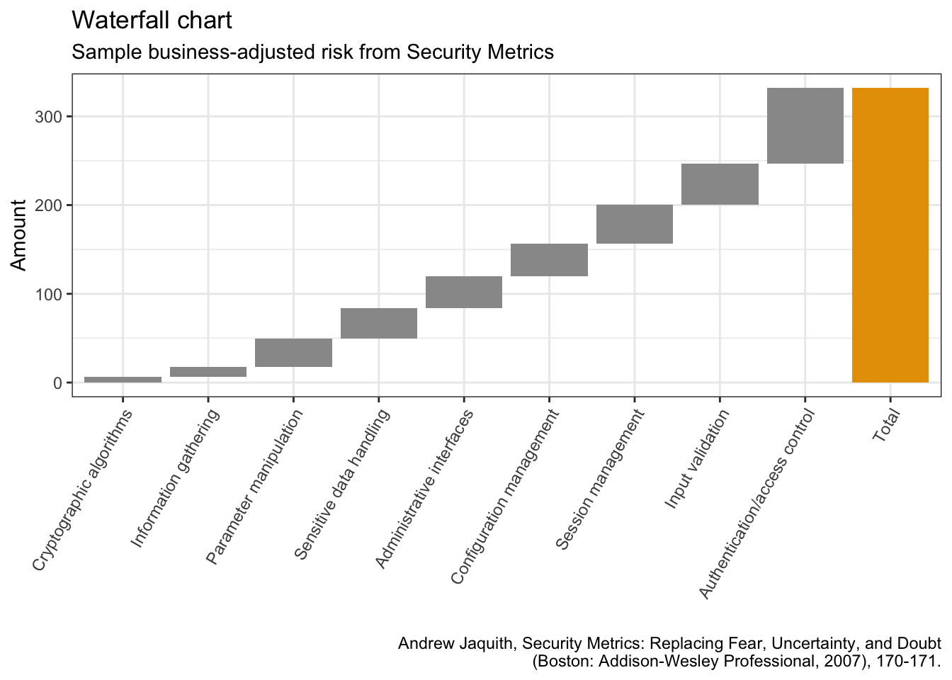
Biplots
library(ggfortify)penguins_prep <- penguins %>%
remove_missing() %>%
select(bill_length_mm:body_mass_g)
penguins_pca <- penguins_prep %>%
prcomp(scale. = TRUE)penguins_km <- penguins_prep %>%
kmeans(3)autoplot(penguins_pca,
data = penguins %>% remove_missing(),
colour = 'species',
shape = 'species',
loadings = TRUE,
loadings.colour = 'blue',
loadings.label = TRUE,
loadings.label.size = 3) +
scale_color_manual(values = cbp1) +
scale_fill_manual(values = cbp1) +
theme_bw() +
labs(
title = "Biplot PCA",
caption = "Source: https://github.com/allisonhorst/palmerpenguins")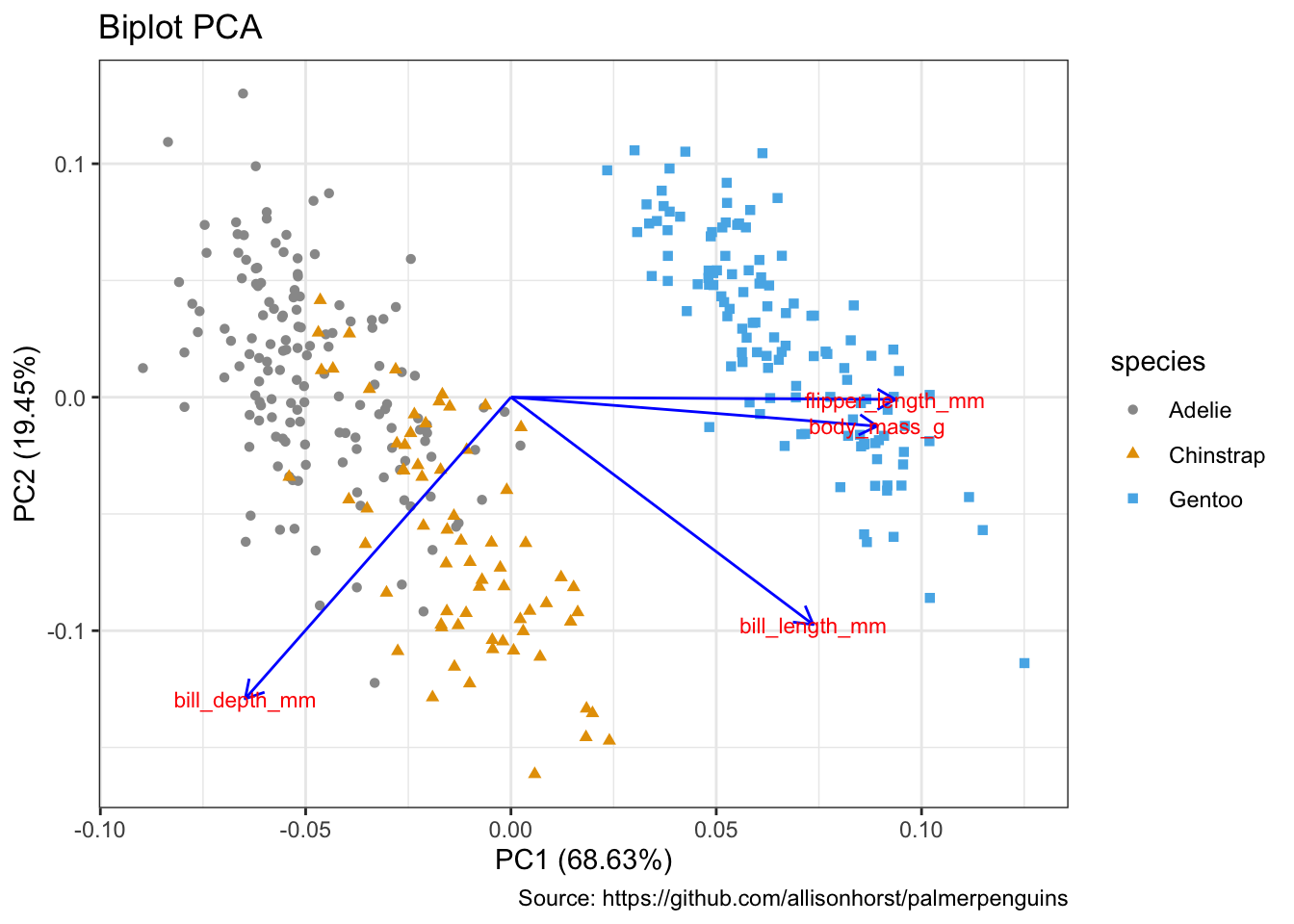
autoplot(penguins_km,
                data = penguins %>% remove_missing(),
                colour = 'species',
                shape = 'species',
                frame = TRUE, frame.type = 'norm') +
      scale_color_manual(values = cbp1) +
  scale_fill_manual(values = cbp1) +
  theme_bw() +
            labs(
            title = "Biplot k-Means clustering",
            caption = "Source: https://github.com/allisonhorst/palmerpenguins")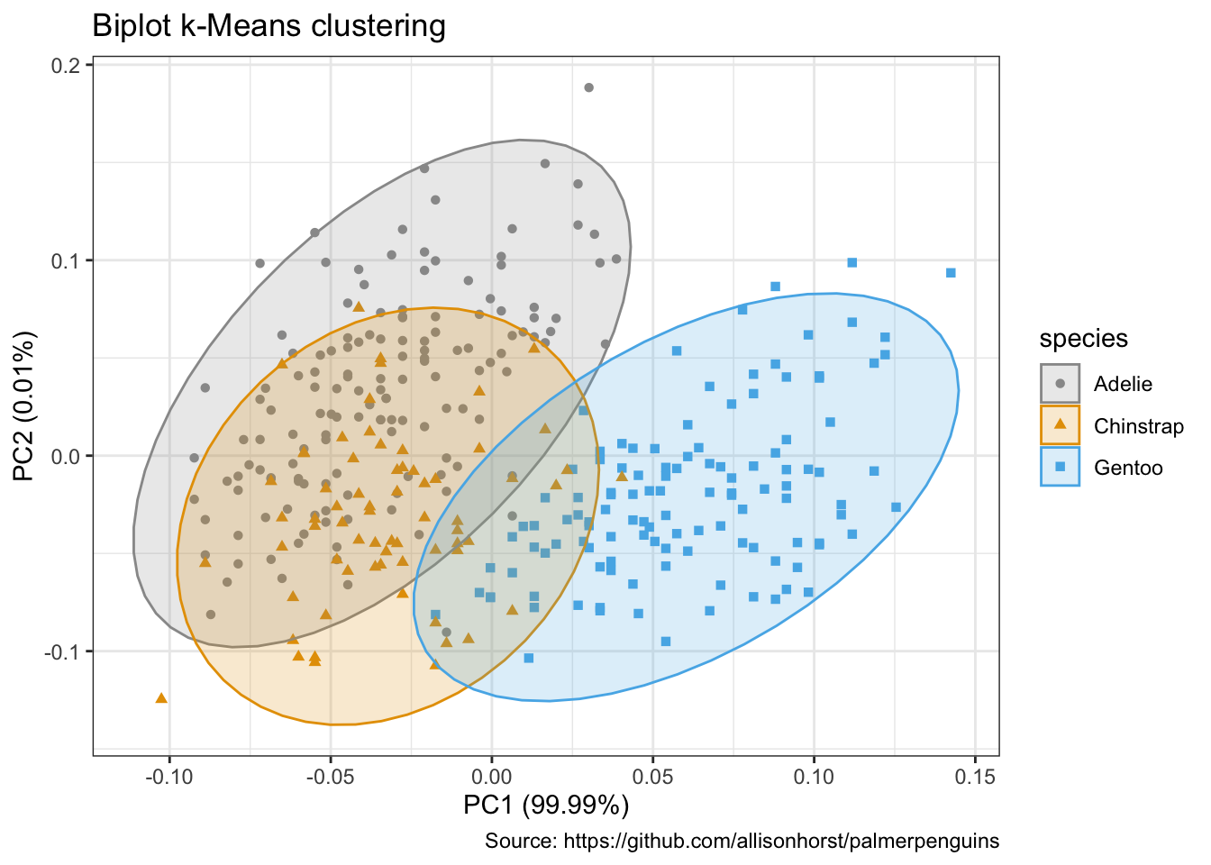
Radar charts, aka star chart, aka spider plot
https://www.data-to-viz.com/caveat/spider.html
library(ggiraphExtra)penguins %>%
remove_missing() %>%
select(-island, -year) %>%
ggRadar(aes(x = c(bill_length_mm, bill_depth_mm, flipper_length_mm, body_mass_g),
group = species,
colour = sex, facet = sex),
rescale = TRUE,
size = 1, interactive = FALSE,
use.label = TRUE) +
scale_color_manual(values = cbp1) +
scale_fill_manual(values = cbp1) +
theme_bw() +
scale_y_discrete(breaks = NULL) + # don't show ticks
labs(
title = "Radar/spider/star chart",
subtitle = "Body mass of male & female penguins per species",
caption = "Source: https://github.com/allisonhorst/palmerpenguins")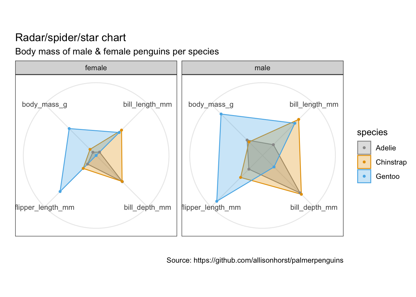
devtools::session_info()## ─ Session info ───────────────────────────────────────────────────────────────
## setting value
## version R version 4.0.2 (2020-06-22)
## os macOS Catalina 10.15.7
## system x86_64, darwin17.0
## ui X11
## language (EN)
## collate en_US.UTF-8
## ctype en_US.UTF-8
## tz Europe/Berlin
## date 2020-10-20
##
## ─ Packages ───────────────────────────────────────────────────────────────────
## package * version date lib source
## ash 1.0-15 2015-09-01 [1] CRAN (R 4.0.2)
## assertthat 0.2.1 2019-03-21 [1] CRAN (R 4.0.0)
## backports 1.1.10 2020-09-15 [1] CRAN (R 4.0.2)
## blob 1.2.1 2020-01-20 [1] CRAN (R 4.0.2)
## blogdown 0.20.1 2020-09-09 [1] Github (rstudio/blogdown@d96fe78)
## bookdown 0.20 2020-06-23 [1] CRAN (R 4.0.2)
## broom 0.7.0 2020-07-09 [1] CRAN (R 4.0.2)
## callr 3.4.4 2020-09-07 [1] CRAN (R 4.0.2)
## cellranger 1.1.0 2016-07-27 [1] CRAN (R 4.0.0)
## cli 2.0.2 2020-02-28 [1] CRAN (R 4.0.0)
## colorspace 1.4-1 2019-03-18 [1] CRAN (R 4.0.0)
## crayon 1.3.4 2017-09-16 [1] CRAN (R 4.0.0)
## DBI 1.1.0 2019-12-15 [1] CRAN (R 4.0.0)
## dbplyr 1.4.4 2020-05-27 [1] CRAN (R 4.0.2)
## dendextend * 1.14.0 2020-08-26 [1] CRAN (R 4.0.2)
## desc 1.2.0 2018-05-01 [1] CRAN (R 4.0.0)
## devtools 2.3.2 2020-09-18 [1] CRAN (R 4.0.2)
## digest 0.6.25 2020-02-23 [1] CRAN (R 4.0.0)
## dplyr * 1.0.2 2020-08-18 [1] CRAN (R 4.0.2)
## ellipsis 0.3.1 2020-05-15 [1] CRAN (R 4.0.0)
## evaluate 0.14 2019-05-28 [1] CRAN (R 4.0.1)
## extrafont 0.17 2014-12-08 [1] CRAN (R 4.0.2)
## extrafontdb 1.0 2012-06-11 [1] CRAN (R 4.0.2)
## fansi 0.4.1 2020-01-08 [1] CRAN (R 4.0.0)
## farver 2.0.3 2020-01-16 [1] CRAN (R 4.0.0)
## fastmap 1.0.1 2019-10-08 [1] CRAN (R 4.0.0)
## forcats * 0.5.0 2020-03-01 [1] CRAN (R 4.0.0)
## fs 1.5.0 2020-07-31 [1] CRAN (R 4.0.2)
## gdtools 0.2.2 2020-04-03 [1] CRAN (R 4.0.2)
## generics 0.0.2 2018-11-29 [1] CRAN (R 4.0.0)
## ggalluvial * 0.12.2 2020-08-30 [1] CRAN (R 4.0.2)
## ggalt * 0.4.0 2017-02-15 [1] CRAN (R 4.0.2)
## ggdendro * 0.1.22 2020-09-13 [1] CRAN (R 4.0.2)
## ggExtra * 0.9 2019-08-27 [1] CRAN (R 4.0.2)
## ggfittext 0.9.0 2020-06-14 [1] CRAN (R 4.0.2)
## ggfortify * 0.4.10 2020-04-26 [1] CRAN (R 4.0.2)
## ggiraph 0.7.8 2020-07-01 [1] CRAN (R 4.0.2)
## ggiraphExtra * 0.2.9 2018-07-22 [1] CRAN (R 4.0.2)
## ggplot2 * 3.3.2 2020-06-19 [1] CRAN (R 4.0.2)
## glue 1.4.2 2020-08-27 [1] CRAN (R 4.0.2)
## gridExtra 2.3 2017-09-09 [1] CRAN (R 4.0.2)
## gtable 0.3.0 2019-03-25 [1] CRAN (R 4.0.0)
## haven 2.3.1 2020-06-01 [1] CRAN (R 4.0.2)
## hms 0.5.3 2020-01-08 [1] CRAN (R 4.0.0)
## htmltools 0.5.0 2020-06-16 [1] CRAN (R 4.0.2)
## htmlwidgets 1.5.1 2019-10-08 [1] CRAN (R 4.0.0)
## httpuv 1.5.4 2020-06-06 [1] CRAN (R 4.0.2)
## httr 1.4.2 2020-07-20 [1] CRAN (R 4.0.2)
## insight 0.9.6 2020-09-20 [1] CRAN (R 4.0.2)
## jsonlite 1.7.1 2020-09-07 [1] CRAN (R 4.0.2)
## KernSmooth 2.23-17 2020-04-26 [1] CRAN (R 4.0.2)
## knitr 1.30 2020-09-22 [1] CRAN (R 4.0.2)
## labeling 0.3 2014-08-23 [1] CRAN (R 4.0.0)
## later 1.1.0.1 2020-06-05 [1] CRAN (R 4.0.2)
## lattice * 0.20-41 2020-04-02 [1] CRAN (R 4.0.2)
## lifecycle 0.2.0 2020-03-06 [1] CRAN (R 4.0.0)
## lubridate 1.7.9 2020-06-08 [1] CRAN (R 4.0.2)
## magrittr 1.5 2014-11-22 [1] CRAN (R 4.0.0)
## maps 3.3.0 2018-04-03 [1] CRAN (R 4.0.2)
## MASS 7.3-53 2020-09-09 [1] CRAN (R 4.0.2)
## Matrix 1.2-18 2019-11-27 [1] CRAN (R 4.0.2)
## memoise 1.1.0 2017-04-21 [1] CRAN (R 4.0.0)
## mgcv 1.8-33 2020-08-27 [1] CRAN (R 4.0.2)
## mime 0.9 2020-02-04 [1] CRAN (R 4.0.0)
## miniUI 0.1.1.1 2018-05-18 [1] CRAN (R 4.0.0)
## modelr 0.1.8 2020-05-19 [1] CRAN (R 4.0.2)
## munsell 0.5.0 2018-06-12 [1] CRAN (R 4.0.0)
## mycor 0.1.1 2018-04-10 [1] CRAN (R 4.0.2)
## nlme 3.1-149 2020-08-23 [1] CRAN (R 4.0.2)
## palmerpenguins * 0.1.0 2020-07-23 [1] CRAN (R 4.0.2)
## pillar 1.4.6 2020-07-10 [1] CRAN (R 4.0.2)
## pkgbuild 1.1.0 2020-07-13 [1] CRAN (R 4.0.2)
## pkgconfig 2.0.3 2019-09-22 [1] CRAN (R 4.0.0)
## pkgload 1.1.0 2020-05-29 [1] CRAN (R 4.0.2)
## plotrix * 3.7-8 2020-04-16 [1] CRAN (R 4.0.2)
## plyr 1.8.6 2020-03-03 [1] CRAN (R 4.0.0)
## ppcor 1.1 2015-12-03 [1] CRAN (R 4.0.2)
## prettyunits 1.1.1 2020-01-24 [1] CRAN (R 4.0.0)
## processx 3.4.4 2020-09-03 [1] CRAN (R 4.0.2)
## proj4 1.0-10 2020-03-02 [1] CRAN (R 4.0.1)
## promises 1.1.1 2020-06-09 [1] CRAN (R 4.0.2)
## ps 1.3.4 2020-08-11 [1] CRAN (R 4.0.2)
## purrr * 0.3.4 2020-04-17 [1] CRAN (R 4.0.0)
## R6 2.4.1 2019-11-12 [1] CRAN (R 4.0.0)
## ragg * 0.3.1 2020-07-03 [1] CRAN (R 4.0.2)
## RColorBrewer 1.1-2 2014-12-07 [1] CRAN (R 4.0.0)
## Rcpp 1.0.5 2020-07-06 [1] CRAN (R 4.0.2)
## readr * 1.3.1 2018-12-21 [1] CRAN (R 4.0.0)
## readxl 1.3.1 2019-03-13 [1] CRAN (R 4.0.0)
## remotes 2.2.0 2020-07-21 [1] CRAN (R 4.0.2)
## reprex 0.3.0 2019-05-16 [1] CRAN (R 4.0.0)
## reshape2 1.4.4 2020-04-09 [1] CRAN (R 4.0.0)
## rlang 0.4.7 2020-07-09 [1] CRAN (R 4.0.2)
## rmarkdown 2.3 2020-06-18 [1] CRAN (R 4.0.2)
## rprojroot 1.3-2 2018-01-03 [1] CRAN (R 4.0.0)
## rstudioapi 0.11 2020-02-07 [1] CRAN (R 4.0.0)
## Rttf2pt1 1.3.8 2020-01-10 [1] CRAN (R 4.0.2)
## rvest 0.3.6 2020-07-25 [1] CRAN (R 4.0.2)
## scales 1.1.1 2020-05-11 [1] CRAN (R 4.0.0)
## sessioninfo 1.1.1 2018-11-05 [1] CRAN (R 4.0.0)
## shiny 1.5.0 2020-06-23 [1] CRAN (R 4.0.2)
## sjlabelled 1.1.7 2020-09-24 [1] CRAN (R 4.0.2)
## sjmisc 2.8.5 2020-05-28 [1] CRAN (R 4.0.2)
## stringi 1.5.3 2020-09-09 [1] CRAN (R 4.0.2)
## stringr * 1.4.0 2019-02-10 [1] CRAN (R 4.0.0)
## systemfonts 0.3.2 2020-09-29 [1] CRAN (R 4.0.2)
## testthat 2.3.2 2020-03-02 [1] CRAN (R 4.0.0)
## tibble * 3.0.3 2020-07-10 [1] CRAN (R 4.0.2)
## tidyr * 1.1.2 2020-08-27 [1] CRAN (R 4.0.2)
## tidyselect 1.1.0 2020-05-11 [1] CRAN (R 4.0.0)
## tidyverse * 1.3.0 2019-11-21 [1] CRAN (R 4.0.0)
## treemapify * 2.5.3 2019-01-30 [1] CRAN (R 4.0.2)
## usethis 1.6.3 2020-09-17 [1] CRAN (R 4.0.2)
## utf8 1.1.4 2018-05-24 [1] CRAN (R 4.0.0)
## uuid 0.1-4 2020-02-26 [1] CRAN (R 4.0.2)
## vctrs 0.3.4 2020-08-29 [1] CRAN (R 4.0.2)
## viridis 0.5.1 2018-03-29 [1] CRAN (R 4.0.2)
## viridisLite 0.3.0 2018-02-01 [1] CRAN (R 4.0.0)
## waterfall * 1.0.2 2016-04-03 [1] CRAN (R 4.0.2)
## withr 2.3.0 2020-09-22 [1] CRAN (R 4.0.2)
## xfun 0.18 2020-09-29 [1] CRAN (R 4.0.2)
## xml2 1.3.2 2020-04-23 [1] CRAN (R 4.0.0)
## xtable 1.8-4 2019-04-21 [1] CRAN (R 4.0.0)
## yaml 2.2.1 2020-02-01 [1] CRAN (R 4.0.0)
##
## [1] /Library/Frameworks/R.framework/Versions/4.0/Resources/library