Data Storytelling presentation

This is code accompanying my talk about Data Storytelling at the German Online Conference Data Science im Unternehmen.

The data has been collected from the Technology Subreddit.

The CSV-file can be found here: https://datanizing.com/data-science-day/transport-short.7z

Or the data can be accessed via this SQLite-databank: https://datanizing.com/data-science-day/technology-transport-short.7z

Libraries

library(readr)
library(tidyverse)
library(tidytext)
library(lubridate)
library(reshape2)

Setting up custom ggplot color scheme

Colorblind-friendly according to https://shirinsplayground.netlify.app/2020/10/goodbadugly/

cbp2 <- c("#000000", "#E69F00", "#56B4E9", "#009E73",
          "#999999", "#0072B2", "#D55E00", "#CC79A7")

ggplot <- function(...) ggplot2::ggplot(...) + 
  scale_color_manual(values = cbp2) +
  scale_fill_manual(values = cbp2) + # note: needs to be overridden when using continuous color scales
  theme_bw()

Reddit API data

https://www.reddit.com/dev/api/

data_reddit <- read_csv(paste0("/Users/shiringlander/Documents/Github/data_storytelling_reddit/", "data/", "transport-short.csv"),
                        col_names = c("id_text_not_null_primary_key", "kind_text", "title_text", "link_id_text", "parent_id_text", "ups_integer", "downs_integer", "score_integer", "author_text", "num_comments", "created_utc_timestamp", "permalink_text", "url_text", "text_text", "level_integer", "top_parent_text"),
                        n_max = Inf) %>%
  mutate(prefix = gsub("(^t.)(_.*)", "\\1", id_text_not_null_primary_key)) %>%
  select(
    id_text_not_null_primary_key,
    prefix,
    link_id_text,
    top_parent_text,
    title_text,
    text_text,
    author_text,
    num_comments,
    ups_integer,
    downs_integer,
    score_integer,
    created_utc_timestamp
         )

data_reddit %>%
  head()

## # A tibble: 6 × 12
##   id_text_not_null_pri… prefix link_id_text top_parent_text title_text text_text
##   <chr>                 <chr>  <chr>        <chr>           <chr>      <chr>    
## 1 t3_kxwsat             t3     <NA>         t3_kxwsat       Rare car …  <NA>    
## 2 t1_gjcnro9            t1     t3_kxwsat    t3_kxwsat       <NA>       "Unfortu…
## 3 t3_kr2ntr             t3     <NA>         t3_kr2ntr       The Devic… "[delete…
## 4 t1_gi73uir            t1     t3_kr2ntr    t3_kr2ntr       <NA>       "Hello! …
## 5 t3_kon7vd             t3     <NA>         t3_kon7vd       Why can't… "[remove…
## 6 t1_ghs2782            t1     t3_kon7vd    t3_kon7vd       <NA>       "Text po…
## # … with 6 more variables: author_text <chr>, num_comments <dbl>,
## #   ups_integer <dbl>, downs_integer <dbl>, score_integer <dbl>,
## #   created_utc_timestamp <dttm>

Prefix types

t1_: Comment
t3_: Link

data_reddit %>%
  count(prefix)

## # A tibble: 2 × 2
##   prefix       n
##   <chr>    <int>
## 1 t1     1272253
## 2 t3       97712

data_reddit_comments <- data_reddit %>%
  filter(prefix == "t1",
         author_text != "[deleted]",
         author_text != "AutoModerator") %>%
  mutate(id = gsub("t1_", "", id_text_not_null_primary_key),
         parent_id = gsub("t._", "", top_parent_text)) %>%
  select(id, parent_id, author_text, text_text, num_comments, ups_integer, downs_integer, score_integer, created_utc_timestamp) %>%
  mutate(date = date(created_utc_timestamp),
         year = year(created_utc_timestamp), 
         month = month(created_utc_timestamp, label = TRUE, abbr = FALSE), 
         wday = wday(created_utc_timestamp, label = TRUE, abbr = FALSE, week_start = 1),
         mday = mday(created_utc_timestamp), 
         hour = hour(created_utc_timestamp),
         time_day = case_when(
           hour > 05 & hour < 8 ~ "a - morgens",
           hour >= 8 & hour < 12 ~ "b - vormittags",
           hour >= 12 & hour < 14 ~ "c - mittags",
           hour >= 14 & hour < 18 ~ "d - nachmittags",
           hour >= 18 & hour < 22 ~ "e - abends",
           hour >=22 | hour <= 5 ~ "f - nachts"))

data_reddit_links <- data_reddit %>%
  filter(prefix == "t3",
         text_text != "[deleted]",
         author_text != "[deleted]",
         text_text != "[removed]") %>%
  mutate(id = gsub("t3_", "", id_text_not_null_primary_key),
         parent_id = gsub("t._", "", top_parent_text)) %>%
  select(id, parent_id, prefix, author_text, title_text, num_comments, ups_integer, downs_integer, score_integer, created_utc_timestamp) %>%
  mutate(date = date(created_utc_timestamp),
         year = year(created_utc_timestamp),
         month = month(created_utc_timestamp, label = TRUE, abbr = FALSE), 
         wday = wday(created_utc_timestamp, label = TRUE, abbr = FALSE, week_start = 1),
         mday = mday(created_utc_timestamp), 
         hour = hour(created_utc_timestamp),
         time_day = case_when(
           hour > 05 & hour < 8 ~ "a - morgens",
           hour >= 8 & hour < 12 ~ "b - vormittags",
           hour >= 12 & hour < 14 ~ "c - mittags",
           hour >= 14 & hour < 18 ~ "d - nachmittags",
           hour >= 18 & hour < 22 ~ "e - abends",
           hour >=22 | hour <= 5 ~ "f - nachts"))

Data stories around timeline

When are comments being posted?

On what date?

data_reddit_comments %>%
  ggplot(aes(x = date)) +
    geom_bar() +
    labs(x = "Datum",
       y = "Anzahl Kommentare",
        title = "Reddit Technology Subreddit", 
        subtitle = "Wie viele Kommentare wurden pro Tag gepostet?",
        caption = "https://www.reddit.com/dev/api/")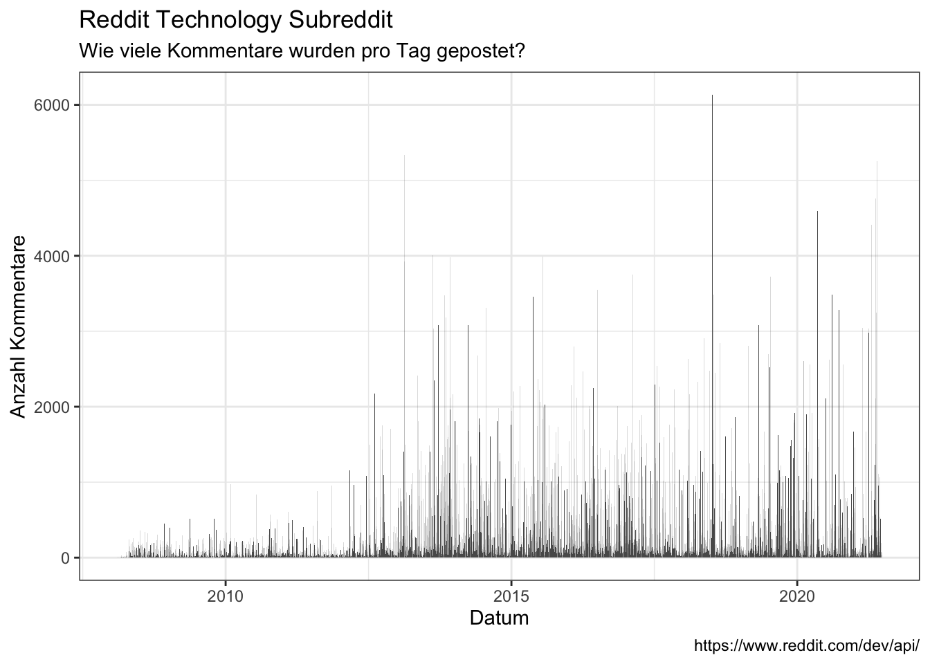

In what year?

data_reddit_comments %>%
  ggplot(aes(x = year)) +
    geom_bar() +
    labs(x = "Jahr",
       y = "Anzahl Kommentare",
        title = "Reddit Technology Subreddit", 
        subtitle = "Wie viele Kommentare wurden pro Jahr gepostet?",
        caption = "https://www.reddit.com/dev/api/")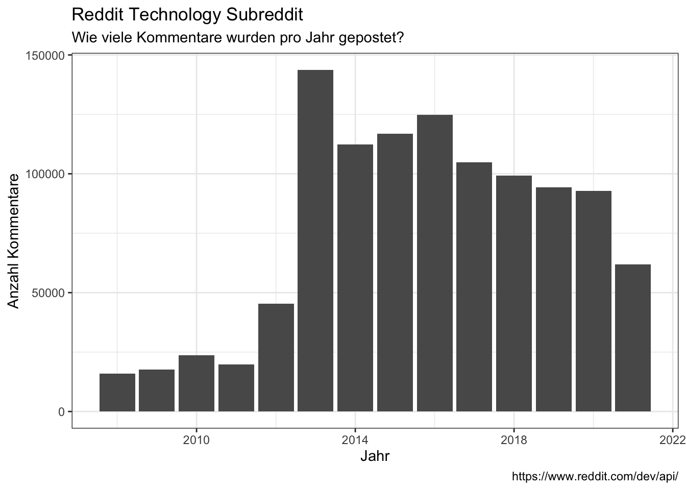

In what month?

data_reddit_comments %>%
  ggplot(aes(x = month)) +
    geom_bar(position = "dodge") +
    labs(x = "Monat",
       y = "Anzahl Kommentare",
        title = "Reddit Technology Subreddit", 
        subtitle = "Wie viele Kommentare wurden pro Monat gepostet?",
        caption = "https://www.reddit.com/dev/api/")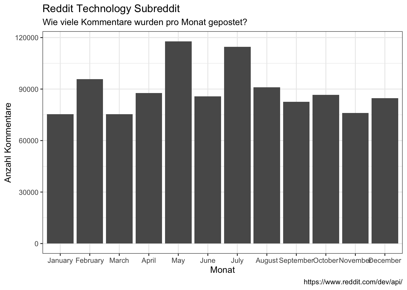

Per month with mean and standard error

data_reddit_comments  %>%
  count(month, year) %>%
  group_by(month) %>% 
  summarize(avg = mean(n),
            sd = sd(n),
            se = sd/sqrt(length((n)))) %>%
  ggplot(aes(x = month, y = avg)) +
    geom_bar(stat = "identity") +
    #geom_errorbar(aes(ymin=avg-sd, ymax=avg+sd)) +
    geom_errorbar(aes(ymin=avg-se, ymax=avg+se), width=0.4) +
    labs(x = "Monat",
       y = "Mittelwert Anzahl Kommentare (+/- Standardfehler)",
        title = "Reddit Technology Subreddit", 
        subtitle = "Wie viele Kommentare wurden pro Monat gepostet?",
        caption = "https://www.reddit.com/dev/api/")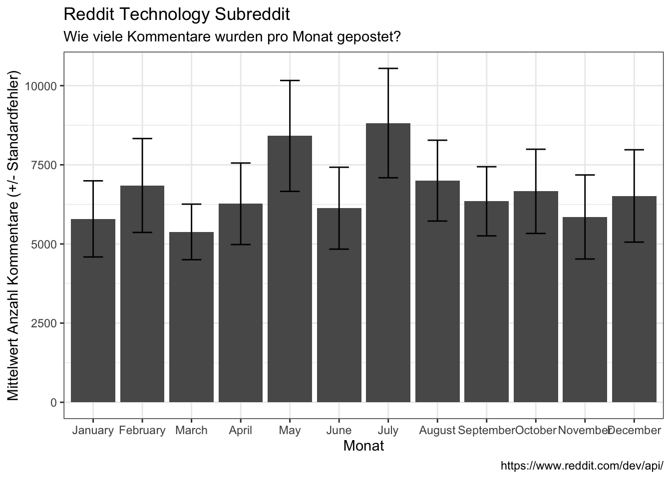

On what weekday?

data_reddit_comments %>%
  ggplot(aes(x = wday)) +
    geom_bar() +
    labs(x = "Wochentag",
       y = "Anzahl Kommentare",
        title = "Reddit Technology Subreddit", 
        subtitle = "Wie viele Kommentare wurden pro Wochentag gepostet?",
        caption = "https://www.reddit.com/dev/api/")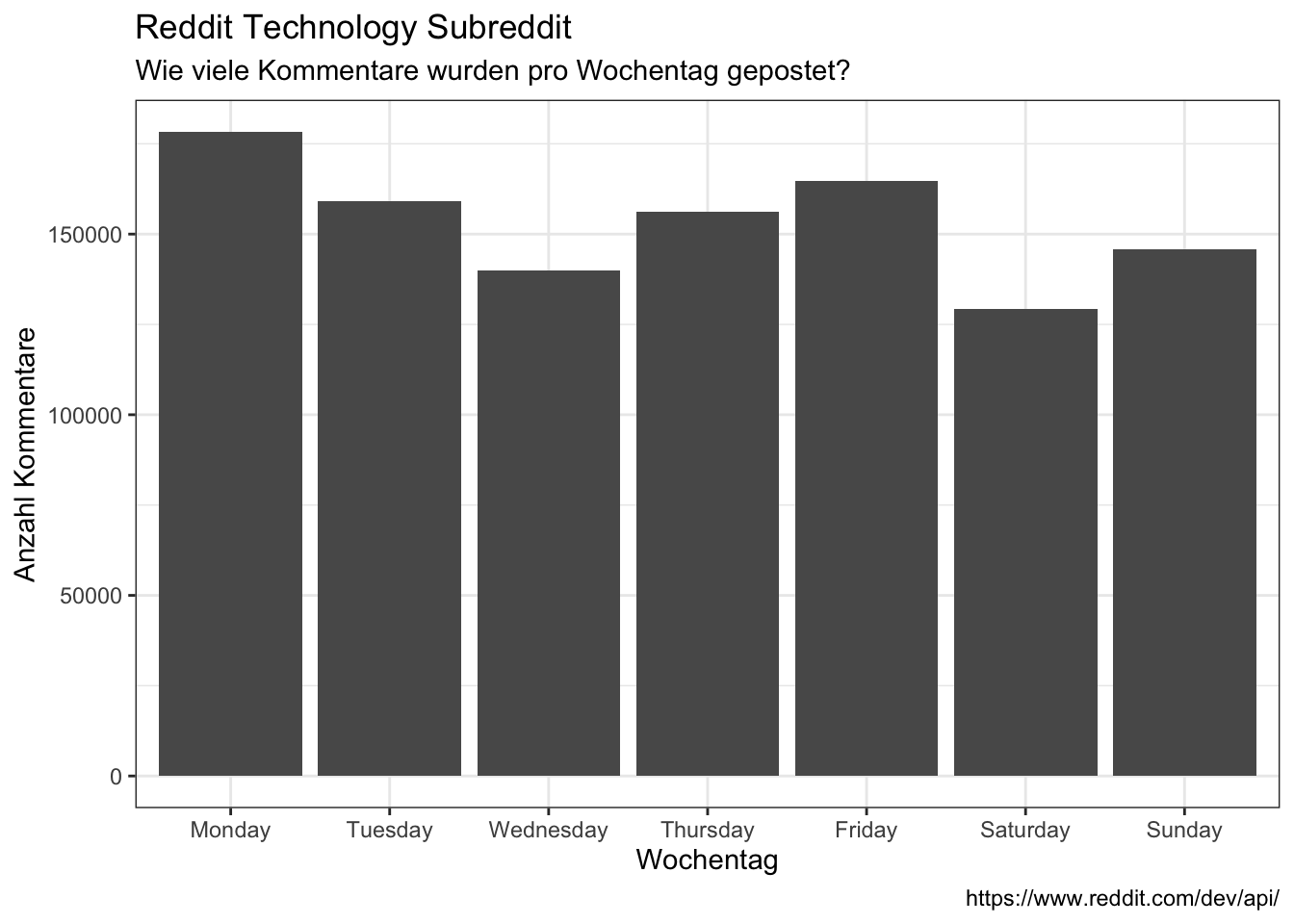

data_reddit_comments %>%
  count(month, wday) %>%
  group_by(wday) %>% 
  summarize(avg = mean(n),
            sd = sd(n),
            se = sd/sqrt(length((n)))) %>%
  ggplot(aes(x = wday, y = avg)) +
    geom_bar(stat = "identity") +
    #geom_errorbar(aes(ymin=avg-sd, ymax=avg+sd)) +
    geom_errorbar(aes(ymin=avg-se, ymax=avg+se), width=0.4) +
    labs(x = "Wochentag",
       y = "Mittelwert Anzahl Kommentare (+/- Standardfehler)",
        title = "Reddit Technology Subreddit", 
        subtitle = "Wie viele Kommentare wurden pro Wochentag gepostet?",
        caption = "https://www.reddit.com/dev/api/")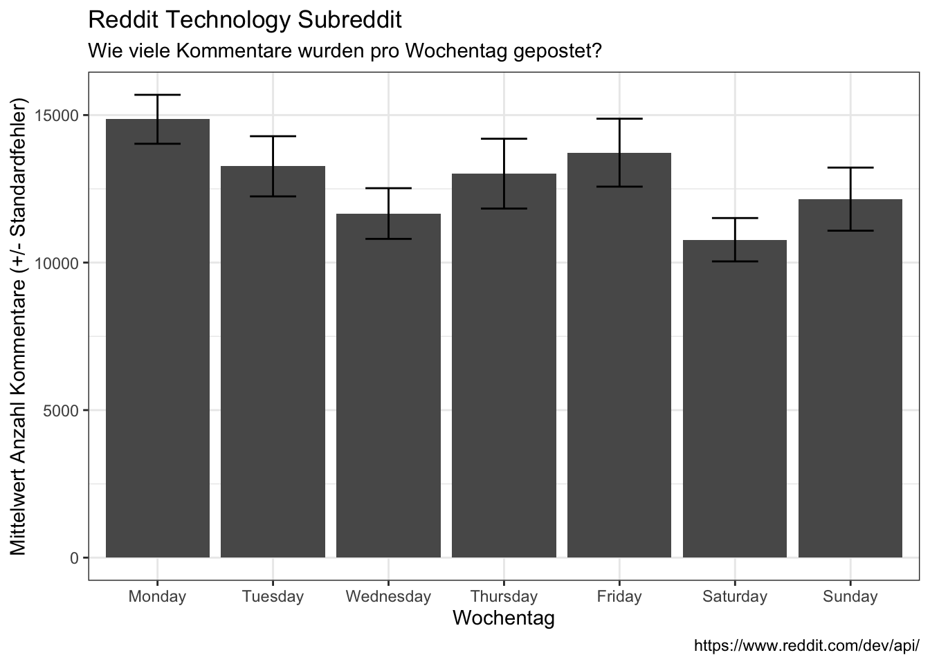

On what time of day?

data_reddit_comments %>%
  ggplot(aes(x = hour, color = time_day, fill = time_day)) +
    geom_bar() +
    labs(x = "Stunde des Tages",
       y = "Anzahl Kommentare",
       color = "Tageszeit",
       fill = "Tageszeit",
        title = "Reddit Technology Subreddit", 
        subtitle = "Wie viele Kommentare wurden pro Stunde des Tages gepostet?",
        caption = "https://www.reddit.com/dev/api/")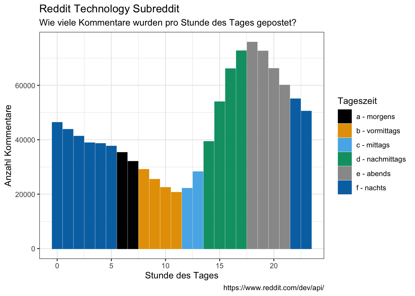

data_reddit_comments %>%
  count(month, hour, time_day) %>%
  group_by(hour, time_day) %>% 
  summarize(avg = mean(n),
            sd = sd(n),
            se = sd/sqrt(length((n)))) %>%
  ggplot(aes(x = hour, y = avg, color = time_day, fill = time_day)) +
    geom_bar(stat = "identity") +
    #geom_errorbar(aes(ymin=avg-sd, ymax=avg+sd)) +
    geom_errorbar(aes(ymin=avg-se, ymax=avg+se), color = "darkgrey", width=0.4) +
    labs(x = "Stunde des Tages",
       y = "Mittelwert Anzahl Kommentare (+/- Standardfehler)",
       color = "Tageszeit",
       fill = "Tageszeit",
        title = "Reddit Technology Subreddit", 
        subtitle = "Wie viele Kommentare wurden pro Stunde des Tages gepostet?",
        caption = "https://www.reddit.com/dev/api/")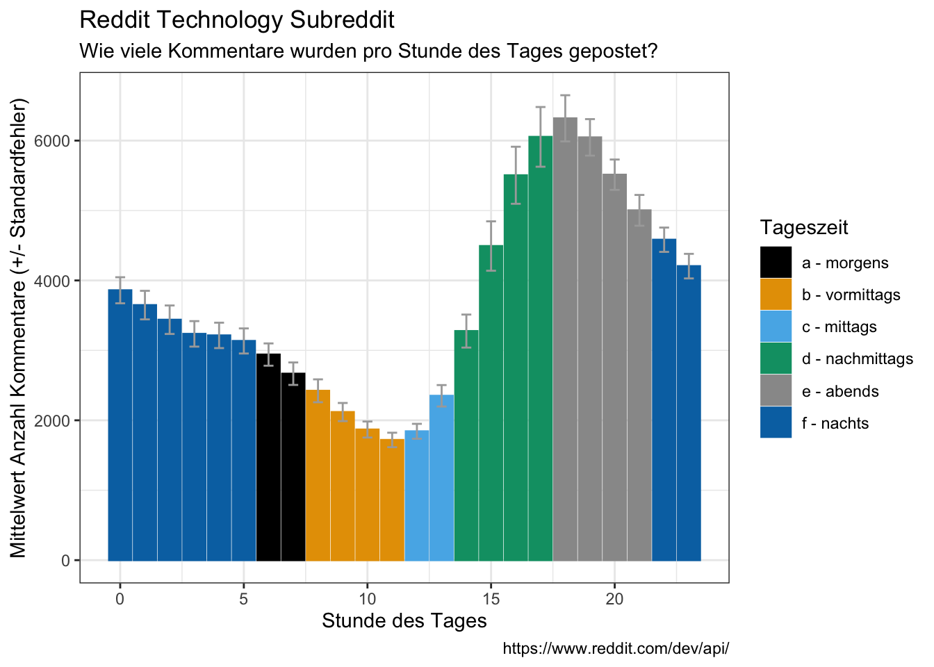

Timezone = UTC

Sentiment analysis

Positivity / negativity

positivity/negativity score of comments over time of day

# scores by time
data_reddit_comments %>%
  group_by(hour, time_day) %>% 
  summarize(avg = mean(score_integer),
            sd = sd(score_integer),
            se = sd/sqrt(length((score_integer)))) %>%
  ggplot(aes(x = hour, y = avg)) +
    geom_line() +
    geom_point(aes(color = time_day)) +
    geom_errorbar(aes(ymin=avg-se, ymax=avg+se, color = time_day), width=0.4) +
    labs(x = "Stunde des Tages",
       y = "Mittelwert Score (Up- vs. Downvotes)",
       color = "Tageszeit",
        title = "Reddit Technology Subreddit", 
        subtitle = "Wie viele Up- vs. Downvotes erhalten Kommentare pro Stunde des Tages?",
        caption = "https://www.reddit.com/dev/api/")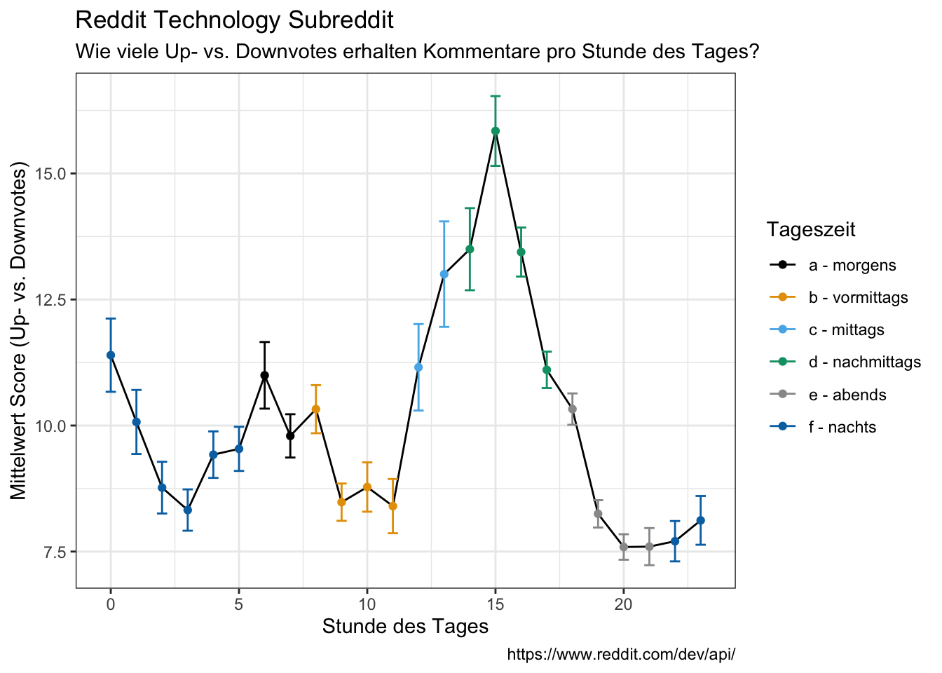

Sentiment data

https://www.tidytextmining.com/

data(stop_words)

tidy_comments <- data_reddit_comments %>%
  mutate(text_text = stringi::stri_enc_toutf8(text_text)) %>%
  unnest_tokens(word, text_text) %>%
  anti_join(stop_words)

#get_sentiments("afinn")
#get_sentiments("bing")
#get_sentiments("nrc")

tidy_comments_bing <- tidy_comments %>%
  inner_join(get_sentiments("bing")) %>%
  group_by(id) %>% 
  count(hour, time_day, sentiment) %>%
  spread(sentiment, n, fill = 0) %>%
  mutate(neg_m_pos = negative - positive,
         neg_by_pos = (negative + 0.0001) / (positive + 0.0001))

tidy_comments_bing %>%
  gather(x, y, negative:positive) %>% 
  group_by(hour, time_day, x) %>%
  summarise(n = sum(y)) %>%
  ggplot(aes(x = hour, y = n, color = x, fill = x)) +
    geom_bar(stat = "identity", position = "dodge", alpha = 0.6) +
    labs(x = "Stunde des Tages",
       y = "Anzahl Kommentare",
       color = "Sentiment",
       fill = "Sentiment",
        title = "Reddit Technology Subreddit", 
        subtitle = "Wie negativ/positiv sind Kommentare über den Tag hinweg?",
        caption = "https://www.reddit.com/dev/api/")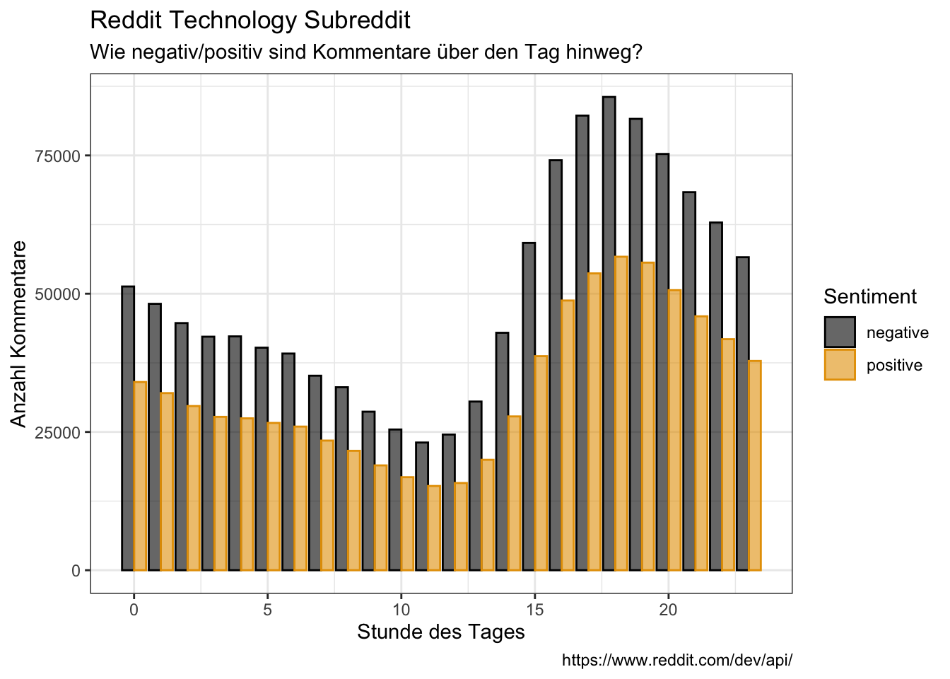

tidy_comments_bing %>%
  group_by(hour, time_day) %>% 
  summarise(mean_neg_m_pos = mean(neg_m_pos)) %>%
  ggplot(aes(hour, mean_neg_m_pos, fill = time_day, color = time_day)) +
  geom_bar(stat = "identity", alpha = 0.6) +
  #coord_flip() +
    labs(x = "Stunde des Tages",
       y = "Sentiment\n(Mw negativer - positiver Score Kommentare)",
       color = "Tageszeit",
       fill = "Tageszeit",
        title = "Reddit Technology Subreddit", 
        subtitle = "Wie negativ/positiv sind Kommentare über den Tag hinweg?",
        caption = "https://www.reddit.com/dev/api/")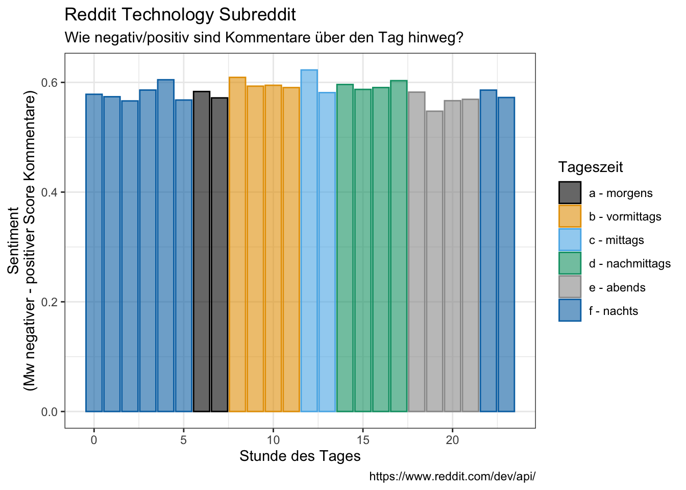

tidy_comments_bing %>%
  group_by(hour, time_day) %>% 
  summarise(mean_neg_by_pos = mean(neg_by_pos)) %>%
  ggplot(aes(hour, mean_neg_by_pos, fill = time_day, color = time_day)) +
  geom_bar(stat = "identity", alpha = 0.6) +
  #coord_flip() +
    labs(x = "Stunde des Tages",
       y = "Sentiment\n(Mw negativer / positiver Score Kommentare)",
       color = "Tageszeit",
       fill = "Tageszeit",
        title = "Reddit Technology Subreddit", 
        subtitle = "Wie negativ/positiv sind Kommentare über den Tag hinweg?",
        caption = "https://www.reddit.com/dev/api/")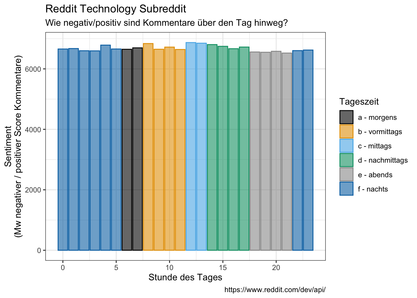

Wordclouds

library(wordcloud)
library(wordcloud2)
library(RColorBrewer)

tidy_comments %>%
  count(word) %>%
  with(wordcloud(word, n, max.words = 100, colors = brewer.pal(8, "Dark2")))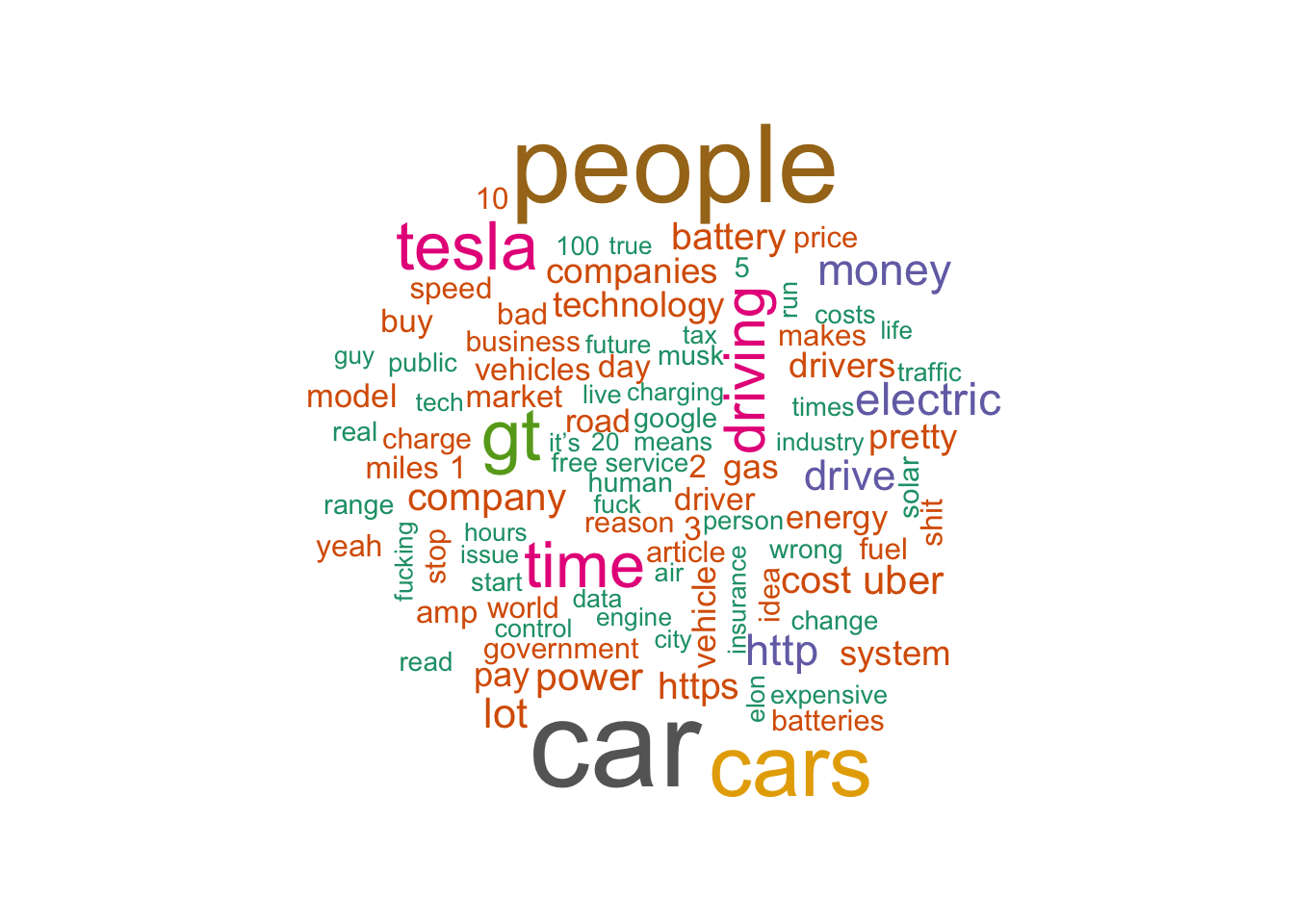

tidy_comments %>%
  count(word) %>%
  wordcloud2(size=1.6, color='random-dark')

tidy_comments %>%
  inner_join(get_sentiments("bing")) %>%
  count(word, sentiment, sort = TRUE) %>%
  acast(word ~ sentiment, value.var = "n", fill = 0) %>%
  comparison.cloud(colors = c("indianred3","lightsteelblue3"),
                   max.words = 100)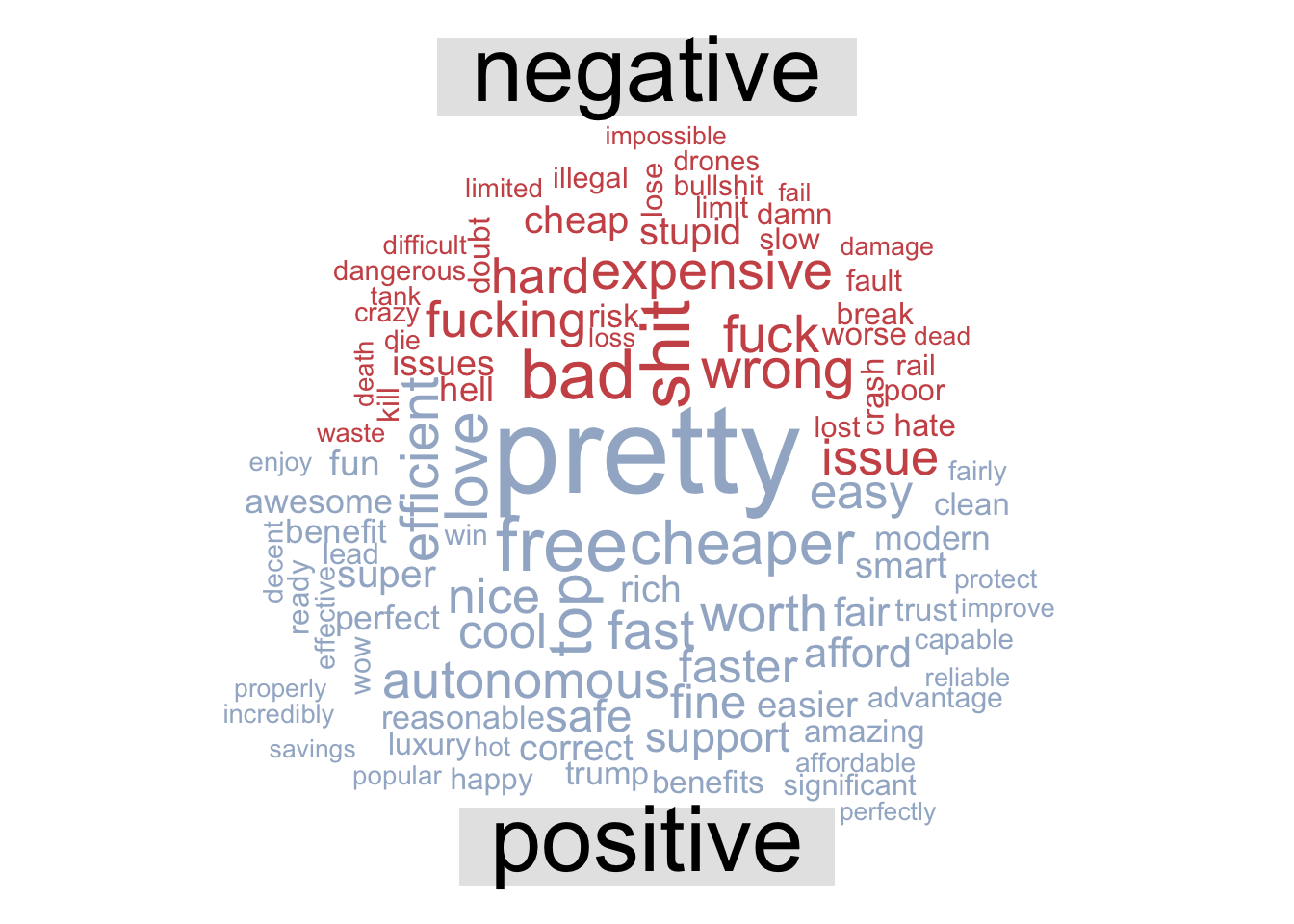

NRC sentiments

tidy_comments_nrc <- tidy_comments %>%
  inner_join(get_sentiments("nrc")) %>%
  group_by(id) %>% 
  count(hour, time_day, sentiment)

tidy_comments_nrc %>%
  group_by(hour, time_day, sentiment) %>% 
  count(sentiment) %>%
  filter(sentiment != "negative",
         sentiment != "positive") %>%
  ggplot(aes(x = hour, y = n, fill = sentiment, color = sentiment)) +
    facet_wrap(vars(sentiment), ncol = 2) +
    geom_bar(stat = "identity", position = "dodge", alpha = 0.6) +
    theme(legend.position = "none") +
    labs(x = "Stunde des Tages",
       y = "Anzahl Kommentare",
        title = "Reddit Technology Subreddit", 
        subtitle = "Welche Sentiments haben Kommentare über den Tag hinweg?",
        caption = "https://www.reddit.com/dev/api/")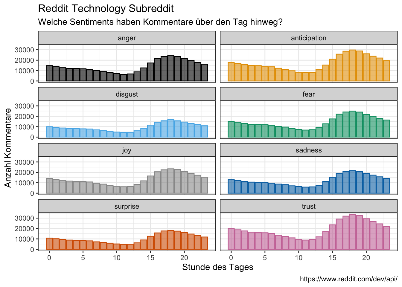

tidy_comments_nrc %>%
  group_by(hour, time_day, sentiment) %>% 
  count(sentiment) %>%
  filter(sentiment != "negative",
         sentiment != "positive") %>%
  group_by(hour, time_day) %>%
  mutate(freq = n / sum(n))%>%
  ggplot(aes(x = hour, y = freq, fill = sentiment, color = sentiment)) +
    geom_bar(stat = "identity", alpha = 0.6) +
    labs(x = "Stunde des Tages",
       y = "Relative Häufigkeit der Kommentare",
        title = "Reddit Technology Subreddit", 
        subtitle = "Welche Sentiments haben Kommentare über den Tag hinweg?",
        caption = "https://www.reddit.com/dev/api/")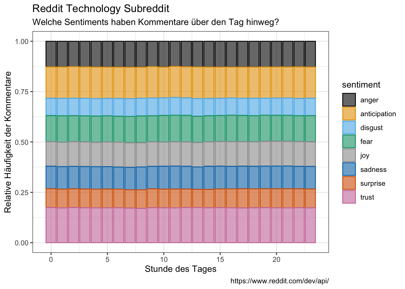

tidy_comments_nrc %>%
  #group_by(hour, time_day, sentiment) %>% 
  #count(sentiment) %>%
  filter(sentiment != "negative",
         sentiment != "positive") %>%
  #group_by(hour, time_day) %>%
  #mutate(freq = n / sum(n))%>%
  ggplot(aes(x = as.factor(hour), y = n, fill = sentiment, color = sentiment)) +
    facet_wrap(vars(time_day), ncol = 2, scales = "free_x") +
    geom_boxplot(alpha = 0.6) +
    labs(x = "Stunde des Tages",
       y = "Relative Häufigkeit der Kommentare",
        title = "Reddit Technology Subreddit", 
        subtitle = "Welche Sentiments haben Kommentare über den Tag hinweg?",
        caption = "https://www.reddit.com/dev/api/")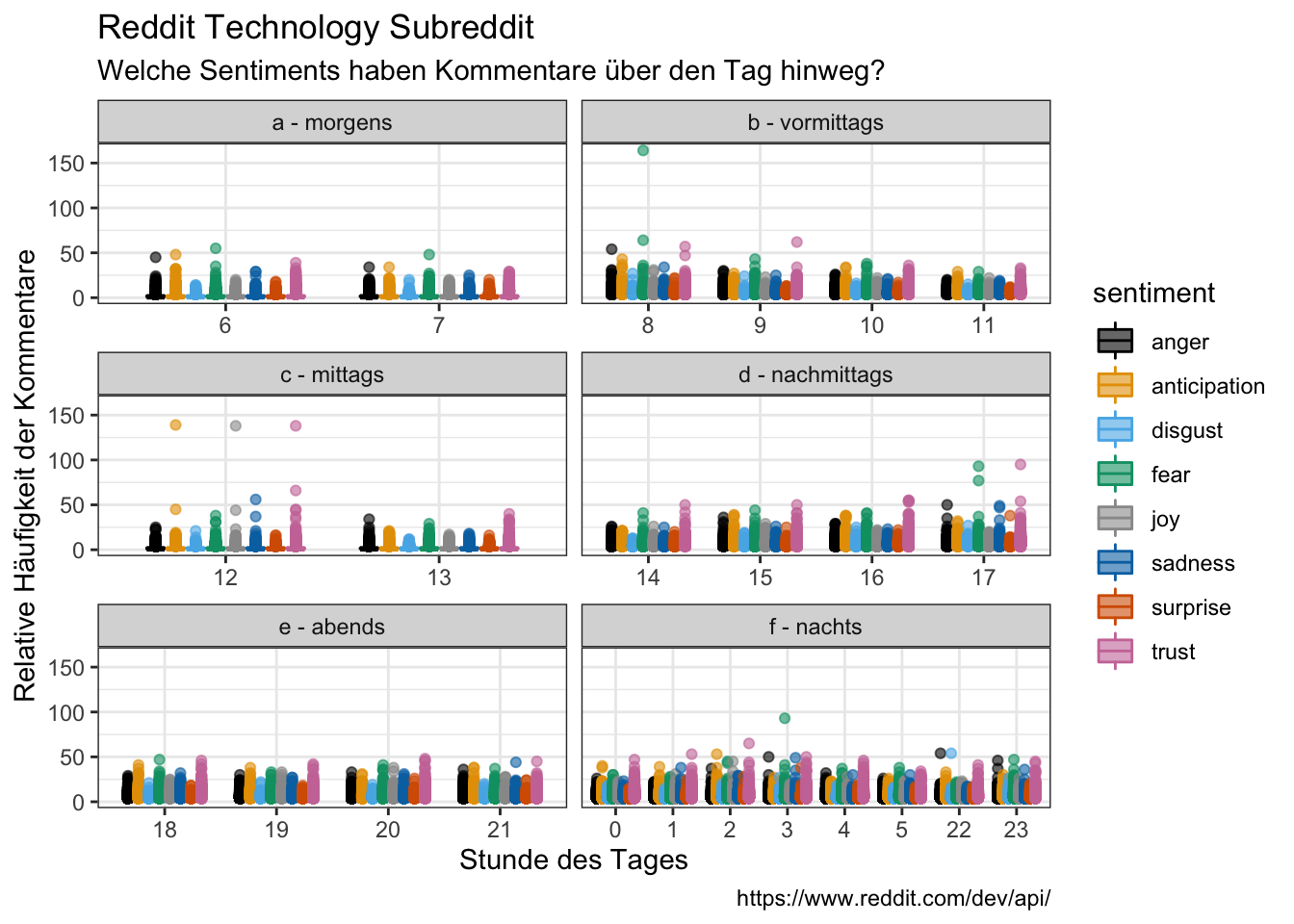

perc <- tidy_comments_nrc %>% 
  filter(sentiment != "negative",
         sentiment != "positive") %>%
  group_by(hour, time_day, sentiment) %>%
  count(hour, time_day, sentiment) %>% 
  ungroup() %>% 
  group_by(hour, time_day) %>%
  mutate(percent = round(n / sum(n) * 100, digits = 2))
  #mutate(labels = scales::percent(perc))

perc %>%
  ggplot(aes(x = "", y = percent, fill = sentiment)) + 
    geom_bar(width = 1, stat = "identity") + 
    theme_minimal() +
    coord_polar("y", start = 0) +
    facet_wrap(vars(hour, time_day), ncol = 8) +
    labs(x = "Stunde des Tages",
       y = "Prozent",
       fill = "Sentiment",
        title = "Reddit Technology Subreddit", 
        subtitle = "Welche Sentiments haben Kommentare über den Tag hinweg?",
        caption = "https://www.reddit.com/dev/api/")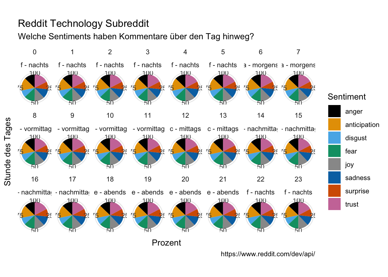

devtools::session_info()

## ─ Session info ───────────────────────────────────────────────────────────────
##  setting  value
##  version  R version 4.1.2 (2021-11-01)
##  os       macOS Big Sur 10.16
##  system   x86_64, darwin17.0
##  ui       X11
##  language (EN)
##  collate  en_US.UTF-8
##  ctype    en_US.UTF-8
##  tz       Europe/Berlin
##  date     2022-04-26
##  pandoc   2.17.1.1 @ /Applications/RStudio.app/Contents/MacOS/quarto/bin/ (via rmarkdown)
## 
## ─ Packages ───────────────────────────────────────────────────────────────────
##  package      * version date (UTC) lib source
##  assertthat     0.2.1   2019-03-21 [1] CRAN (R 4.1.0)
##  backports      1.4.1   2021-12-13 [1] CRAN (R 4.1.0)
##  bit            4.0.4   2020-08-04 [1] CRAN (R 4.1.0)
##  bit64          4.0.5   2020-08-30 [1] CRAN (R 4.1.0)
##  blogdown       1.9     2022-03-28 [1] CRAN (R 4.1.2)
##  bookdown       0.25    2022-03-16 [1] CRAN (R 4.1.2)
##  brio           1.1.3   2021-11-30 [1] CRAN (R 4.1.0)
##  broom          0.7.12  2022-01-28 [1] CRAN (R 4.1.2)
##  bslib          0.3.1   2021-10-06 [1] CRAN (R 4.1.0)
##  cachem         1.0.6   2021-08-19 [1] CRAN (R 4.1.0)
##  callr          3.7.0   2021-04-20 [1] CRAN (R 4.1.0)
##  cellranger     1.1.0   2016-07-27 [1] CRAN (R 4.1.0)
##  cli            3.2.0   2022-02-14 [1] CRAN (R 4.1.2)
##  colorspace     2.0-3   2022-02-21 [1] CRAN (R 4.1.2)
##  crayon         1.5.1   2022-03-26 [1] CRAN (R 4.1.2)
##  DBI            1.1.2   2021-12-20 [1] CRAN (R 4.1.0)
##  dbplyr         2.1.1   2021-04-06 [1] CRAN (R 4.1.0)
##  desc           1.4.1   2022-03-06 [1] CRAN (R 4.1.2)
##  devtools       2.4.3   2021-11-30 [1] CRAN (R 4.1.0)
##  digest         0.6.29  2021-12-01 [1] CRAN (R 4.1.0)
##  dplyr        * 1.0.8   2022-02-08 [1] CRAN (R 4.1.2)
##  ellipsis       0.3.2   2021-04-29 [1] CRAN (R 4.1.0)
##  evaluate       0.15    2022-02-18 [1] CRAN (R 4.1.2)
##  fansi          1.0.3   2022-03-24 [1] CRAN (R 4.1.2)
##  farver         2.1.0   2021-02-28 [1] CRAN (R 4.1.0)
##  fastmap        1.1.0   2021-01-25 [1] CRAN (R 4.1.0)
##  forcats      * 0.5.1   2021-01-27 [1] CRAN (R 4.1.0)
##  fs             1.5.2   2021-12-08 [1] CRAN (R 4.1.0)
##  generics       0.1.2   2022-01-31 [1] CRAN (R 4.1.2)
##  ggplot2      * 3.3.5   2021-06-25 [1] CRAN (R 4.1.0)
##  glue           1.6.2   2022-02-24 [1] CRAN (R 4.1.2)
##  gtable         0.3.0   2019-03-25 [1] CRAN (R 4.1.0)
##  haven          2.4.3   2021-08-04 [1] CRAN (R 4.1.0)
##  highr          0.9     2021-04-16 [1] CRAN (R 4.1.0)
##  hms            1.1.1   2021-09-26 [1] CRAN (R 4.1.0)
##  htmltools      0.5.2   2021-08-25 [1] CRAN (R 4.1.0)
##  htmlwidgets    1.5.4   2021-09-08 [1] CRAN (R 4.1.0)
##  httr           1.4.2   2020-07-20 [1] CRAN (R 4.1.0)
##  janeaustenr    0.1.5   2017-06-10 [1] CRAN (R 4.1.0)
##  jquerylib      0.1.4   2021-04-26 [1] CRAN (R 4.1.0)
##  jsonlite       1.8.0   2022-02-22 [1] CRAN (R 4.1.2)
##  knitr          1.38    2022-03-25 [1] CRAN (R 4.1.2)
##  labeling       0.4.2   2020-10-20 [1] CRAN (R 4.1.0)
##  lattice        0.20-45 2021-09-22 [1] CRAN (R 4.1.2)
##  lifecycle      1.0.1   2021-09-24 [1] CRAN (R 4.1.1)
##  lubridate    * 1.8.0   2021-10-07 [1] CRAN (R 4.1.0)
##  magrittr       2.0.3   2022-03-30 [1] CRAN (R 4.1.2)
##  Matrix         1.4-1   2022-03-23 [1] CRAN (R 4.1.2)
##  memoise        2.0.1   2021-11-26 [1] CRAN (R 4.1.0)
##  modelr         0.1.8   2020-05-19 [1] CRAN (R 4.1.0)
##  munsell        0.5.0   2018-06-12 [1] CRAN (R 4.1.0)
##  pillar         1.7.0   2022-02-01 [1] CRAN (R 4.1.2)
##  pkgbuild       1.3.1   2021-12-20 [1] CRAN (R 4.1.0)
##  pkgconfig      2.0.3   2019-09-22 [1] CRAN (R 4.1.0)
##  pkgload        1.2.4   2021-11-30 [1] CRAN (R 4.1.0)
##  plyr           1.8.7   2022-03-24 [1] CRAN (R 4.1.2)
##  prettyunits    1.1.1   2020-01-24 [1] CRAN (R 4.1.0)
##  processx       3.5.3   2022-03-25 [1] CRAN (R 4.1.2)
##  ps             1.6.0   2021-02-28 [1] CRAN (R 4.1.0)
##  purrr        * 0.3.4   2020-04-17 [1] CRAN (R 4.1.0)
##  R6             2.5.1   2021-08-19 [1] CRAN (R 4.1.0)
##  rappdirs       0.3.3   2021-01-31 [1] CRAN (R 4.1.0)
##  RColorBrewer * 1.1-3   2022-04-03 [1] CRAN (R 4.1.2)
##  Rcpp           1.0.8.3 2022-03-17 [1] CRAN (R 4.1.2)
##  readr        * 2.1.2   2022-01-30 [1] CRAN (R 4.1.2)
##  readxl         1.4.0   2022-03-28 [1] CRAN (R 4.1.2)
##  remotes        2.4.2   2021-11-30 [1] CRAN (R 4.1.0)
##  reprex         2.0.1   2021-08-05 [1] CRAN (R 4.1.0)
##  reshape2     * 1.4.4   2020-04-09 [1] CRAN (R 4.1.0)
##  rlang          1.0.2   2022-03-04 [1] CRAN (R 4.1.2)
##  rmarkdown      2.13    2022-03-10 [1] CRAN (R 4.1.2)
##  rprojroot      2.0.3   2022-04-02 [1] CRAN (R 4.1.2)
##  rstudioapi     0.13    2020-11-12 [1] CRAN (R 4.1.0)
##  rvest          1.0.2   2021-10-16 [1] CRAN (R 4.1.0)
##  sass           0.4.1   2022-03-23 [1] CRAN (R 4.1.2)
##  scales         1.1.1   2020-05-11 [1] CRAN (R 4.1.0)
##  sessioninfo    1.2.2   2021-12-06 [1] CRAN (R 4.1.0)
##  SnowballC      0.7.0   2020-04-01 [1] CRAN (R 4.1.0)
##  stringi        1.7.6   2021-11-29 [1] CRAN (R 4.1.0)
##  stringr      * 1.4.0   2019-02-10 [1] CRAN (R 4.1.0)
##  testthat       3.1.3   2022-03-29 [1] CRAN (R 4.1.2)
##  textdata       0.4.1   2020-05-04 [1] CRAN (R 4.1.0)
##  tibble       * 3.1.6   2021-11-07 [1] CRAN (R 4.1.0)
##  tidyr        * 1.2.0   2022-02-01 [1] CRAN (R 4.1.2)
##  tidyselect     1.1.2   2022-02-21 [1] CRAN (R 4.1.2)
##  tidytext     * 0.3.2   2021-09-30 [1] CRAN (R 4.1.0)
##  tidyverse    * 1.3.1   2021-04-15 [1] CRAN (R 4.1.0)
##  tokenizers     0.2.1   2018-03-29 [1] CRAN (R 4.1.0)
##  tzdb           0.3.0   2022-03-28 [1] CRAN (R 4.1.2)
##  usethis        2.1.5   2021-12-09 [1] CRAN (R 4.1.0)
##  utf8           1.2.2   2021-07-24 [1] CRAN (R 4.1.0)
##  vctrs          0.4.0   2022-03-30 [1] CRAN (R 4.1.2)
##  vroom          1.5.7   2021-11-30 [1] CRAN (R 4.1.0)
##  withr          2.5.0   2022-03-03 [1] CRAN (R 4.1.2)
##  wordcloud    * 2.6     2018-08-24 [1] CRAN (R 4.1.0)
##  wordcloud2   * 0.2.1   2018-01-03 [1] CRAN (R 4.1.0)
##  xfun           0.30    2022-03-02 [1] CRAN (R 4.1.2)
##  xml2           1.3.3   2021-11-30 [1] CRAN (R 4.1.0)
##  yaml           2.3.5   2022-02-21 [1] CRAN (R 4.1.2)
## 
##  [1] /Library/Frameworks/R.framework/Versions/4.1/Resources/library
## 
## ──────────────────────────────────────────────────────────────────────────────

Data Storytelling presentation

Libraries

Setting up custom ggplot color scheme

Reddit API data

Prefix types

Data stories around timeline

When are comments being posted?

Sentiment analysis

Positivity / negativity

Sentiment data

Wordclouds

NRC sentiments

Dr. Shirin Elsinghorst