
Using Keras Callbacks
This is article #3 in my recent series on how to get the most out of Keras. The two other articles are:
- Update with TF 2.0: Image classification with Keras and TensorFlow
- Whose dream is this? When and how to use the Keras Functional API
Keras comes with a number of built in callbacks. Callbacks are useful for optimizing/customizing your training runs and are used with the fit() function. Here, I’ll show which callbacks come built into Keras and how to write your own custom callbacks.
Workshop announcement: Because this year’s UseR 2020 in Munich couldn’t happen as an in-person event, I will be giving my workshop on Deep Learning with Keras and TensorFlow as an online event on Thursday, 8th of October (13:00 UTC / 15:00 CEST). You can register for FREE via Eventbrite.
If you have questions or would like to talk about this article (or something else data-related), you can now book 15-minute timeslots with me (it’s free - one slot available per weekday):

If you have been enjoying my content and would like to help me be able to create more, please consider sending me a donation at . Thank you! :-)
Note:
I have been having an issue with blogdown, where the code below runs perfectly fine in my R console from within the RMarkdown file but whenever I include any function from the keras package, blogdown::serve_site() throws an error: Error in render_page(f) : Failed to render 'content/post/keras.Rmd'.
Since I have no idea what’s going on there (blogdown::serve_site() builds my site without trouble as long as I don’t include keras functions) and haven’t gotten a reply to the issue I posted to Github, I had to write this blogpost without actually running the code while building the site.
I worked around that problem by not evaluating most of the code below and instead ran the code locally on my computer. Objects and images, I then saved as .RData or .png files and manually put them back into the document. By just reading this blogpost as it rendered on my site, you won’t notice much of a difference (except where I copy/pasted the output as comments below the code) but in order to be fully transparent, you can see on Github what I did with hidden code chunks to create this post.
# load libraries
library(tidyverse)
library(tensorflow)
library(keras)
# check TF version
tf_version()
#[1] ‘2.2’
# check if keras is available
is_keras_available()
#[1] TRUEModel setup
The setup part remains unchanged compared to before.
# path to image folders
train_image_files_path <- "/fruits/Training/"
# list of fruits to modle
fruit_list <- c("Kiwi", "Banana", "Apricot", "Avocado", "Cocos", "Clementine", "Mandarine", "Orange",
"Limes", "Lemon", "Peach", "Plum", "Raspberry", "Strawberry", "Pineapple", "Pomegranate")
# number of output classes (i.e. fruits)
output_n <- length(fruit_list)
# image size to scale down to (original images are 100 x 100 px)
img_width <- 20
img_height <- 20
target_size <- c(img_width, img_height)
# RGB = 3 channels
channels <- 3
# define batch size
batch_size <- 32train_data_gen <- image_data_generator(
rescale = 1/255,
validation_split = 0.3)# training images
train_image_array_gen <- flow_images_from_directory(train_image_files_path,
train_data_gen,
subset = 'training',
target_size = target_size,
class_mode = "categorical",
classes = fruit_list,
batch_size = batch_size,
seed = 42)
#Found 5401 images belonging to 16 classes.
# validation images
valid_image_array_gen <- flow_images_from_directory(train_image_files_path,
train_data_gen,
subset = 'validation',
target_size = target_size,
class_mode = "categorical",
classes = fruit_list,
batch_size = batch_size,
seed = 42)
#Found 2308 images belonging to 16 classes.- One change is that I’ll be increasing the number of epochs to 100. Don’t worry, we won’t actually train our model for 100 epochs, this is just to demonstrate how early stopping works. ;-)
# number of training samples
train_samples <- train_image_array_gen$n
# number of validation samples
valid_samples <- valid_image_array_gen$n

# define number of epochs
epochs <- 100
# input layer
inputs <- layer_input(shape = c(img_width, img_height, channels))
# outputs compose input + dense layers
predictions <- inputs %>%
layer_conv_2d(filter = 32, kernel_size = c(3,3), padding = "same") %>%
layer_activation("relu") %>%
# Second hidden layer
layer_conv_2d(filter = 16, kernel_size = c(3,3), padding = "same") %>%
layer_activation_leaky_relu(0.5) %>%
layer_batch_normalization() %>%
# Use max pooling
layer_max_pooling_2d(pool_size = c(2,2)) %>%
layer_dropout(0.25) %>%
# Flatten max filtered output into feature vector
# and feed into dense layer
layer_flatten() %>%
layer_dense(100) %>%
layer_activation("relu") %>%
layer_dropout(0.5) %>%
# Outputs from dense layer are projected onto output layer
layer_dense(output_n) %>%
layer_activation("softmax")Callbacks
You can find a list of all callbacks on CRAN. Let’s look at each one in turn:
Early stopping
The early-stopping callback is by far my most often utilized callback when training Keras functions. Usually, you want to stop training once training and validation loss no longer improve (significantly) and before you begin overfitting your model. But after how many epochs is that? You could of course start training and judge by eye, then stop training and set the number of epochs to your desired size before training your final model.
A more elegant and practical approach is to set the number of epochs much higher than you think you’ll need and have the early-stopping callback handle the rest for you. You can tell callback_early_stopping what metric to monitor for improvements (usually, you want to look at the validation loss if you have a validation set), how much this metric has to change in order to be counted as “model still improves” (min_delta) and after how many epochs with no improvement training should stop (patience).
Here, I also set restore_best_weights = TRUE, so that the weights from the best model (aka from the epoch with lowest validation loss) will be restored.
early_stop <- callback_early_stopping(monitor = "val_loss",
                                      min_delta = 0.001,
                                      patience = 5,
                                      restore_best_weights = TRUE,
                                      verbose = 1)
Checkpoints
Usually, you’ll want to save your final model after training but you can also (additionally) save models during training. The callback_model_checkpoint saves a model after every epoch (default) or you can choose to only save a model if it’s performance is better than that from the epoch before (save_best_only = TRUE). You can even include epoch number and performance metric in the file name.
save_cp <- callback_model_checkpoint("../../../keras_model_cps/checkpoints/weights.{epoch:02d}-{val_loss:.2f}.hdf5",
                                     monitor = "val_loss",
                                     save_best_only = TRUE,
                                     verbose = 1)
Adjusting the learning rate
Adjusting the learning rate of the optimizer during training (as opposed to using a fixed learning rate throughout the entire training process) is often used to improve the final model performance. Usually, you will reduce the learning rate during training as that means that you’ll start out by taking big steps (aka weight changes) in the general “right direction” (in short: you are looking for the global minimum in your error landscape = your target) and once you get closer to your target, you’ll take smaller steps so as not to miss the target and get as close to it as possible (fine-tuning weights). But both reduction and increase of the learning rate can help you overcome local minima or saddle points in the error landscape.
We can use two callbacks to adjust the learning rate:
callback_learning_rate_scheduler
This callback takes a function with epoch number and learning rate as input. You’ll define how to change the learning rate depending on the epoch number and return the new learning rate as the function output. Here you’ll see two examples for a learning rate scheduler:
- In this scheduler, you will start with a fixed learning rate (defined later with
model %>% compile()) and use that for the first 10 epochs. After the 10th epoch, you’ll reduce the learning rate every other epoch.
lr_schedule_1 <- function(epoch, lr) {

  if (epoch <= 10) {

    return(lr)

  } else {

    if (epoch %% 2 == 0) {
      return(lr * tf$math$exp(-0.1))
    }
  }
}

reduce_lr_1 <- callback_learning_rate_scheduler(lr_schedule_1)- Alternatively, you can define a decay rate and have the learning rate reduced by this decay rate on every decay step (e.g. every second epoch).
lr_schedule_2 <- function(epoch, lr) {

  decay_rate = 0.1
  decay_step = 2

  if (epoch %% decay_step == 0) {
    lr * decay_rate
  }

  return(lr)

}

reduce_lr_2 <- callback_learning_rate_scheduler(lr_schedule_2)
Of course, you can change the learning rate any which way you want and that seems useful to you. However, finding a good learning rate curve isn’t trivial, so I tend to use the following callback instead:
callback_reduce_lr_on_plateau
This callback will reduce the learning rate once your model stagnates (i.e. when the performance metric doesn’t improve any more). This callback monitors a performance metric for improvements again, just as the callback_early_stopping callback above. The difference here is that training won’t stop once the monitored metric doesn’t improve for a given number of epochs but instead the learning rate is reduced by a given factor.
reduce_lr_pt <- callback_reduce_lr_on_plateau(
  monitor = "val_loss",
  factor = 0.1,
  patience = 5,
  min_lr = 0.0000001,
  verbose = 1
)
Terminate training on NA
This callback is pretty simple and self-explanatory: it will stop training if the loss is NA.
terminate_na <- callback_terminate_on_naan()Logging
The logging callback is essentially the progress bar you will see in your standard-out (usually the console) during training. With callback_progbar_logger you can customize this progess bar. See the function help for more info.
prog_bar <- callback_progbar_logger(count_mode = "steps")CSV logger
The callback_csv_logger will write epoch results to log files in csv format. We’ll look at the output of this csv-file below after finishing training.
logfile <- callback_csv_logger("../../../keras_model_cps/run/log.csv")TensorBoard
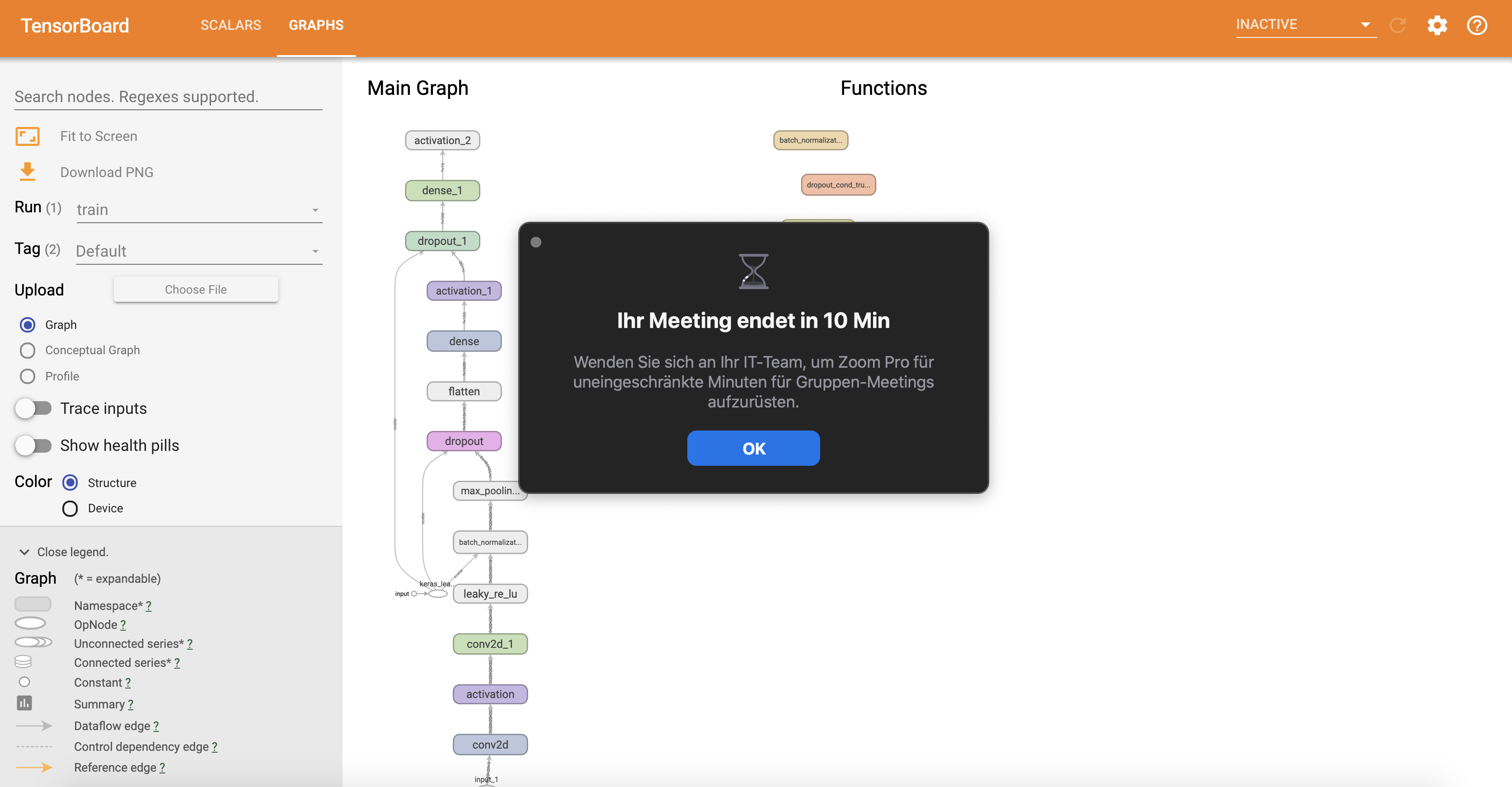
TensorBoard is the TensorFlow visualization framework and as such can only be used if you are training with the TensorFlow backend. During training, you’ll want to be able to see what’s going on with the training process: Is it still running? Is the loss improving? By how much is it improving What epoch are we on? Etc.
To do good research or develop good models, you need rich, frequent feedback about what’s going on inside your models during your experiments. That’s the point of running experiments: to get information about how well a model performs—as much information as possible. Making progress is an iterative process, or loop: you start with an idea and express it as an experiment, attempting to validate or invalidate your idea. You run this experiment and process the information it generates. This inspires your next idea. The more iterations of this loop you’re able to run, the more refined and powerful your ideas become. Keras helps you go from idea to experiment in the least possible time, and fast GPUs can help you get from experiment to result as quickly as possible. But what about processing the experiment results? That’s where Tensor-Board comes in.
This section introduces TensorBoard, a browser-based visualization tool that comes packaged with TensorFlow. Note that it’s only available for Keras models when you’re using Keras with the TensorFlow backend.
The key purpose of TensorBoard is to help you visually monitor everything that goes on inside your model during training. If you’re monitoring more information than just the model’s final loss, you can develop a clearer vision of what the model does and doesn’t do, and you can make progress more quickly. TensorBoard gives you access to several neat features, all in your browser:
Visually monitoring metrics during training Visualizing your model architecture Visualizing histograms of activations and gradients Exploring embeddings in 3D Let’s demonstrate these features on a simple example. You’ll train a 1D convnet on the IMDB sentiment-analysis task.
tensorboard <- callback_tensorboard("../../../keras_model_cps/logs")Remote monitoring
remote_monitor <- callback_remote_monitor(
  root = "http://localhost:9000",
  path = "../../../keras_model_cps/publish/epoch/end/",
  field = "data",
  headers = NULL,
  send_as_json = FALSE
)
Writing your own callback
You can create a custom callback by creating a new R6 class that inherits from the KerasCallback class.
If you need to take a specific action during training that isn’t covered by one of the built-in callbacks, you can write your own callback. Callbacks are implemented by creating a new R6 class that inherits from the KerasCallback class. You can then implement any number of the following transparently named methods, which are called at various points during training:
1 Called at the start of every epoch 2 Called at the end of every epoch 3 Called right before processing each batch 4 Called right after processing each batch 5 Called at the start of training 6 Called at the end of training These methods all are called with a logs argument, which is a named list containing information about the previous batch, epoch, or training run: training and validation metrics, and so on. Additionally, the callback has access to the following attributes:
self\(model—Reference to the Keras model being trained self\)params—Named list with training parameters (verbosity, batch size, number of epochs, and so on) Here’s a simple example that saves a list of losses over each batch during training:
1 Called at the end of every training batch 2 Accumulates losses from every batch in a list 3 Creates an instance of the callback 4 Attaches the callback to model training 5 Accumulated losses are now available from the callback instance.
# define custom callback class
LossHistory <- R6::R6Class("LossHistory",
  inherit = KerasCallback,

  public = list(

    losses = NULL,

    on_batch_end = function(batch, logs = list()) {
      self$losses <- c(self$losses, logs[["loss"]])
    }
))

# define model
model <- keras_model_sequential()

# add layers and compile
model %>%
  layer_dense(units = 10, input_shape = c(784)) %>%
  layer_activation(activation = 'softmax') %>%
  compile(
    loss = 'categorical_crossentropy',
    optimizer = 'rmsprop'
  )

# create history callback object and use it during training
history <- LossHistory$new()
model %>% fit(
  X_train, Y_train,
  batch_size=128, epochs=20, verbose=0,
  callbacks= list(history)
)

# print the accumulated losses
history$losses
custom_cb <- callback_lambda(
#on_train_begin = function(self, logs = NULL) {
# keys = list(logs.keys())
# cat("\nStarting training; got log keys:", keys)
#},
on_epoch_begin = function(self, epoch, logs = NULL) {
#if (epoch %% 5 == 0) {
print("\nEpoch", {epoch:02d}, "start\n")
#}
},
on_epoch_end = function(self, epoch, logs = NULL) {
print("The average loss for {epoch:02d} is {val_loss:.2f}") #and mean absolute error is", logs["mean_absolute_error"])
}#,
#on_train_end = function(self, logs = NULL) {
# keys = list(logs.keys())
# cat("\nStop training; got log keys:", keys)
#}
)Model training with callbacks
# create and compile model
model <- keras_model(inputs = inputs,
                     outputs = predictions) %>%
  compile(
  loss = "categorical_crossentropy",
  optimizer = optimizer_rmsprop(lr = 0.0001, decay = 1e-6),
  metrics = "accuracy"
)

hist <- model %>%

  fit_generator(
  # training data
  train_image_array_gen,

  # epochs
  steps_per_epoch = as.integer(train_samples / batch_size),
  epochs = epochs,

  # validation data
  validation_data = valid_image_array_gen,
  validation_steps = as.integer(valid_samples / batch_size),

  # callbacks
  callbacks = list(
    early_stop,
    terminate_na,
    save_cp,
    logfile,
    tensorboard#,
    #reduce_lr,
    #reduce_lr_pt,
    #remote_monitor,
    #custom_cb
  )
)
Epoch 1/100
168/168 [==============================] - 20s 117ms/step - loss: 2.1054 - accuracy: 0.3278 - val_loss: 2.0478 - val_accuracy: 0.6059
Epoch 2/100
168/168 [==============================] - 14s 86ms/step - loss: 1.0841 - accuracy: 0.6374 - val_loss: 0.9194 - val_accuracy: 0.8924
Epoch 3/100
168/168 [==============================] - 10s 62ms/step - loss: 0.6357 - accuracy: 0.7905 - val_loss: 0.3312 - val_accuracy: 0.9240
Epoch 4/100
168/168 [==============================] - 11s 67ms/step - loss: 0.4122 - accuracy: 0.8650 - val_loss: 0.1618 - val_accuracy: 0.9692
Epoch 5/100
168/168 [==============================] - 11s 68ms/step - loss: 0.2736 - accuracy: 0.9162 - val_loss: 0.0921 - val_accuracy: 0.9822
Epoch 6/100
168/168 [==============================] - 13s 80ms/step - loss: 0.2064 - accuracy: 0.9376 - val_loss: 0.0798 - val_accuracy: 0.9805
Epoch 7/100
168/168 [==============================] - 11s 64ms/step - loss: 0.1446 - accuracy: 0.9536 - val_loss: 0.0687 - val_accuracy: 0.9818
Epoch 8/100
168/168 [==============================] - 11s 65ms/step - loss: 0.1128 - accuracy: 0.9668 - val_loss: 0.0366 - val_accuracy: 0.9896
Epoch 9/100
168/168 [==============================] - 10s 62ms/step - loss: 0.0839 - accuracy: 0.9752 - val_loss: 0.0376 - val_accuracy: 0.9852
Epoch 10/100
168/168 [==============================] - 11s 65ms/step - loss: 0.0761 - accuracy: 0.9782 - val_loss: 0.0340 - val_accuracy: 0.9891
Epoch 11/100
168/168 [==============================] - 10s 60ms/step - loss: 0.0631 - accuracy: 0.9823 - val_loss: 0.0351 - val_accuracy: 0.9878
Epoch 12/100
168/168 [==============================] - 11s 63ms/step - loss: 0.0499 - accuracy: 0.9849 - val_loss: 0.0155 - val_accuracy: 0.9965
Epoch 13/100
168/168 [==============================] - 10s 61ms/step - loss: 0.0434 - accuracy: 0.9888 - val_loss: 0.0174 - val_accuracy: 0.9948
Epoch 14/100
168/168 [==============================] - 13s 75ms/step - loss: 0.0360 - accuracy: 0.9907 - val_loss: 0.0170 - val_accuracy: 0.9926
Epoch 15/100
168/168 [==============================] - 12s 70ms/step - loss: 0.0339 - accuracy: 0.9892 - val_loss: 0.0148 - val_accuracy: 0.9944
Epoch 16/100
168/168 [==============================] - 15s 87ms/step - loss: 0.0299 - accuracy: 0.9922 - val_loss: 0.0186 - val_accuracy: 0.9926
Epoch 17/100
168/168 [==============================] - 12s 74ms/step - loss: 0.0252 - accuracy: 0.9931 - val_loss: 0.0099 - val_accuracy: 0.9978
Epoch 18/100
168/168 [==============================] - 10s 58ms/step - loss: 0.0238 - accuracy: 0.9940 - val_loss: 0.0185 - val_accuracy: 0.9909
Epoch 19/100
168/168 [==============================] - 10s 58ms/step - loss: 0.0220 - accuracy: 0.9935 - val_loss: 0.0063 - val_accuracy: 1.0000
Epoch 20/100
168/168 [==============================] - 10s 58ms/step - loss: 0.0233 - accuracy: 0.9922 - val_loss: 0.0108 - val_accuracy: 0.9957
Epoch 21/100
168/168 [==============================] - 10s 60ms/step - loss: 0.0173 - accuracy: 0.9957 - val_loss: 0.0308 - val_accuracy: 0.9887
Epoch 22/100
168/168 [==============================] - 10s 59ms/step - loss: 0.0162 - accuracy: 0.9953 - val_loss: 0.0161 - val_accuracy: 0.9939
Epoch 23/100
168/168 [==============================] - 10s 58ms/step - loss: 0.0160 - accuracy: 0.9953 - val_loss: 0.0060 - val_accuracy: 0.9974
Epoch 24/100
168/168 [==============================] - 10s 59ms/step - loss: 0.0176 - accuracy: 0.9944 - val_loss: 0.0055 - val_accuracy: 0.9983histhist_csv <- readr::read_csv("../../../keras_model_cps/run/log.csv")
hist_csv %>%
gather("x", "y", accuracy:val_loss) %>%
mutate(y = as.numeric(y),
metric = gsub("val_", "", x),
set = case_when(
grepl("val", x, fixed = TRUE) ~ "validation",
TRUE ~ "training")) %>%
ggplot(aes(x = epoch, y = y, color = set)) +
facet_wrap(vars(metric), ncol = 1, scales = "free_y") +
geom_line() +
geom_point()tensorboard("../../../keras_model_cps/logs")Started TensorBoard at http://127.0.0.1:4302 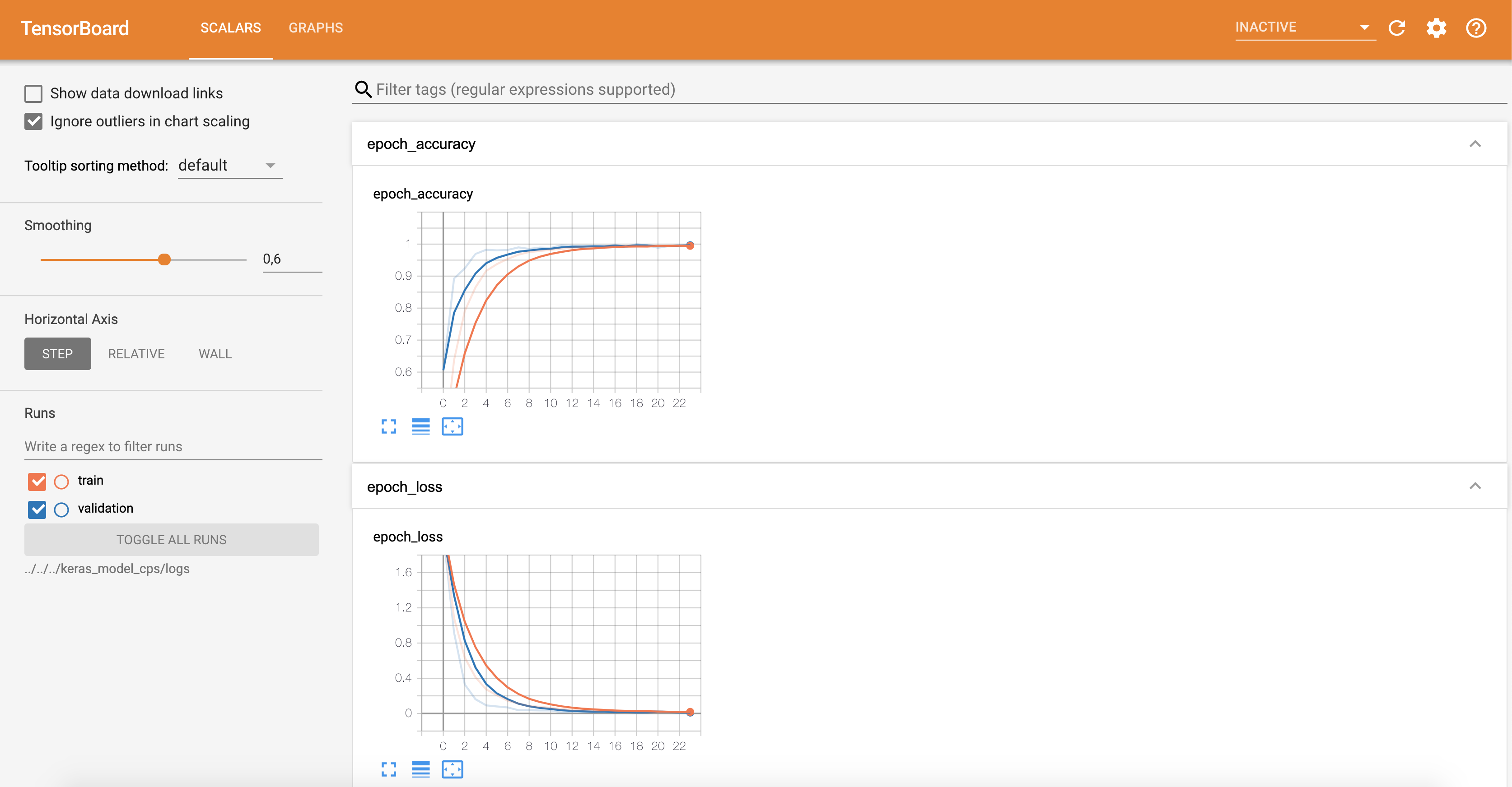
devtools::session_info()## ─ Session info ───────────────────────────────────────────────────────────────
## setting value
## version R version 4.0.2 (2020-06-22)
## os macOS Catalina 10.15.7
## system x86_64, darwin17.0
## ui X11
## language (EN)
## collate en_US.UTF-8
## ctype en_US.UTF-8
## tz Europe/Berlin
## date 2020-10-19
##
## ─ Packages ───────────────────────────────────────────────────────────────────
## package * version date lib source
## assertthat 0.2.1 2019-03-21 [1] CRAN (R 4.0.0)
## backports 1.1.10 2020-09-15 [1] CRAN (R 4.0.2)
## base64enc 0.1-3 2015-07-28 [1] CRAN (R 4.0.0)
## blob 1.2.1 2020-01-20 [1] CRAN (R 4.0.2)
## blogdown 0.20.1 2020-09-09 [1] Github (rstudio/blogdown@d96fe78)
## bookdown 0.20 2020-06-23 [1] CRAN (R 4.0.2)
## broom 0.7.0 2020-07-09 [1] CRAN (R 4.0.2)
## callr 3.4.4 2020-09-07 [1] CRAN (R 4.0.2)
## cellranger 1.1.0 2016-07-27 [1] CRAN (R 4.0.0)
## cli 2.0.2 2020-02-28 [1] CRAN (R 4.0.0)
## colorspace 1.4-1 2019-03-18 [1] CRAN (R 4.0.0)
## crayon 1.3.4 2017-09-16 [1] CRAN (R 4.0.0)
## DBI 1.1.0 2019-12-15 [1] CRAN (R 4.0.0)
## dbplyr 1.4.4 2020-05-27 [1] CRAN (R 4.0.2)
## desc 1.2.0 2018-05-01 [1] CRAN (R 4.0.0)
## devtools 2.3.2 2020-09-18 [1] CRAN (R 4.0.2)
## digest 0.6.25 2020-02-23 [1] CRAN (R 4.0.0)
## dplyr * 1.0.2 2020-08-18 [1] CRAN (R 4.0.2)
## ellipsis 0.3.1 2020-05-15 [1] CRAN (R 4.0.0)
## evaluate 0.14 2019-05-28 [1] CRAN (R 4.0.1)
## fansi 0.4.1 2020-01-08 [1] CRAN (R 4.0.0)
## forcats * 0.5.0 2020-03-01 [1] CRAN (R 4.0.0)
## fs 1.5.0 2020-07-31 [1] CRAN (R 4.0.2)
## generics 0.0.2 2018-11-29 [1] CRAN (R 4.0.0)
## ggplot2 * 3.3.2 2020-06-19 [1] CRAN (R 4.0.2)
## glue 1.4.2 2020-08-27 [1] CRAN (R 4.0.2)
## gtable 0.3.0 2019-03-25 [1] CRAN (R 4.0.0)
## haven 2.3.1 2020-06-01 [1] CRAN (R 4.0.2)
## hms 0.5.3 2020-01-08 [1] CRAN (R 4.0.0)
## htmltools 0.5.0 2020-06-16 [1] CRAN (R 4.0.2)
## httr 1.4.2 2020-07-20 [1] CRAN (R 4.0.2)
## jsonlite 1.7.1 2020-09-07 [1] CRAN (R 4.0.2)
## keras * 2.3.0.0.9000 2020-09-15 [1] Github (rstudio/keras@ad737d1)
## knitr 1.30 2020-09-22 [1] CRAN (R 4.0.2)
## lattice 0.20-41 2020-04-02 [1] CRAN (R 4.0.2)
## lifecycle 0.2.0 2020-03-06 [1] CRAN (R 4.0.0)
## lubridate 1.7.9 2020-06-08 [1] CRAN (R 4.0.2)
## magrittr 1.5 2014-11-22 [1] CRAN (R 4.0.0)
## Matrix 1.2-18 2019-11-27 [1] CRAN (R 4.0.2)
## memoise 1.1.0 2017-04-21 [1] CRAN (R 4.0.0)
## modelr 0.1.8 2020-05-19 [1] CRAN (R 4.0.2)
## munsell 0.5.0 2018-06-12 [1] CRAN (R 4.0.0)
## pillar 1.4.6 2020-07-10 [1] CRAN (R 4.0.2)
## pkgbuild 1.1.0 2020-07-13 [1] CRAN (R 4.0.2)
## pkgconfig 2.0.3 2019-09-22 [1] CRAN (R 4.0.0)
## pkgload 1.1.0 2020-05-29 [1] CRAN (R 4.0.2)
## prettyunits 1.1.1 2020-01-24 [1] CRAN (R 4.0.0)
## processx 3.4.4 2020-09-03 [1] CRAN (R 4.0.2)
## ps 1.3.4 2020-08-11 [1] CRAN (R 4.0.2)
## purrr * 0.3.4 2020-04-17 [1] CRAN (R 4.0.0)
## R6 2.4.1 2019-11-12 [1] CRAN (R 4.0.0)
## Rcpp 1.0.5 2020-07-06 [1] CRAN (R 4.0.2)
## readr * 1.3.1 2018-12-21 [1] CRAN (R 4.0.0)
## readxl 1.3.1 2019-03-13 [1] CRAN (R 4.0.0)
## remotes 2.2.0 2020-07-21 [1] CRAN (R 4.0.2)
## reprex 0.3.0 2019-05-16 [1] CRAN (R 4.0.0)
## reticulate 1.16-9001 2020-09-15 [1] Github (rstudio/reticulate@4f6a898)
## rlang 0.4.7 2020-07-09 [1] CRAN (R 4.0.2)
## rmarkdown 2.3 2020-06-18 [1] CRAN (R 4.0.2)
## rprojroot 1.3-2 2018-01-03 [1] CRAN (R 4.0.0)
## rstudioapi 0.11 2020-02-07 [1] CRAN (R 4.0.0)
## rvest 0.3.6 2020-07-25 [1] CRAN (R 4.0.2)
## scales 1.1.1 2020-05-11 [1] CRAN (R 4.0.0)
## sessioninfo 1.1.1 2018-11-05 [1] CRAN (R 4.0.0)
## stringi 1.5.3 2020-09-09 [1] CRAN (R 4.0.2)
## stringr * 1.4.0 2019-02-10 [1] CRAN (R 4.0.0)
## tensorflow * 2.2.0 2020-05-11 [1] CRAN (R 4.0.2)
## testthat 2.3.2 2020-03-02 [1] CRAN (R 4.0.0)
## tfruns 1.4 2018-08-25 [1] CRAN (R 4.0.0)
## tibble * 3.0.3 2020-07-10 [1] CRAN (R 4.0.2)
## tidyr * 1.1.2 2020-08-27 [1] CRAN (R 4.0.2)
## tidyselect 1.1.0 2020-05-11 [1] CRAN (R 4.0.0)
## tidyverse * 1.3.0 2019-11-21 [1] CRAN (R 4.0.0)
## usethis 1.6.3 2020-09-17 [1] CRAN (R 4.0.2)
## vctrs 0.3.4 2020-08-29 [1] CRAN (R 4.0.2)
## whisker 0.4 2019-08-28 [1] CRAN (R 4.0.0)
## withr 2.3.0 2020-09-22 [1] CRAN (R 4.0.2)
## xfun 0.18 2020-09-29 [1] CRAN (R 4.0.2)
## xml2 1.3.2 2020-04-23 [1] CRAN (R 4.0.0)
## yaml 2.2.1 2020-02-01 [1] CRAN (R 4.0.0)
## zeallot 0.1.0 2018-01-28 [1] CRAN (R 4.0.0)
##
## [1] /Library/Frameworks/R.framework/Versions/4.0/Resources/library
