Spreading a Passion for R with the Münster Community in Germany Recently, I gave an interview to the RConsortium talking about my motivation to start the MünsteR useR-group.
You can read the interview here.
This is code accompanying my talk about Data Storytelling at the German Online Conference Data Science im Unternehmen.
The data has been collected from the Technology Subreddit.
The CSV-file can be found here: https://datanizing.com/data-science-day/transport-short.7z
Or the data can be accessed via this SQLite-databank: https://datanizing.com/data-science-day/technology-transport-short.7z
Libraries library(readr) library(tidyverse) library(tidytext) library(lubridate) library(reshape2) Setting up custom ggplot color scheme Colorblind-friendly according to https://shirinsplayground.netlify.app/2020/10/goodbadugly/ cbp2 <- c("#000000", "#E69F00", "#56B4E9", "#009E73", "#999999", "#0072B2", "#D55E00", "#CC79A7") ggplot <- function(.
This is code accompanying an article about Data Storytelling in the German IT magazine iX 1/2022. The figures in this article were created as follows.
Note: Because the data is partly from a German source, the data description is in German as well.
iX 1/2022
library(readr) library(tidyverse) library(stringr) library(lubridate) Set colorblind-friendly palette cbp2 <- c("#000000", "#E69F00", "#56B4E9", "#009E73", "#999999", "#0072B2", "#D55E00", "#CC79A7") ggplot <- function(...) ggplot2::ggplot(...) + scale_color_manual(values = cbp2) + scale_fill_manual(values = cbp2) + # note: needs to be overridden when using continuous color scales theme_bw() library(plotrix) sliceValues <- rep(10, 8) # each slice value=10 for proportionate slices ( p <- pie3D(sliceValues, explode=0, theta = 1.
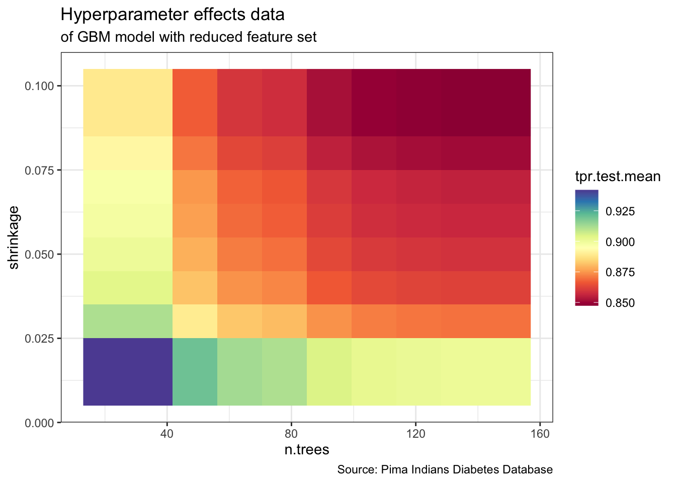
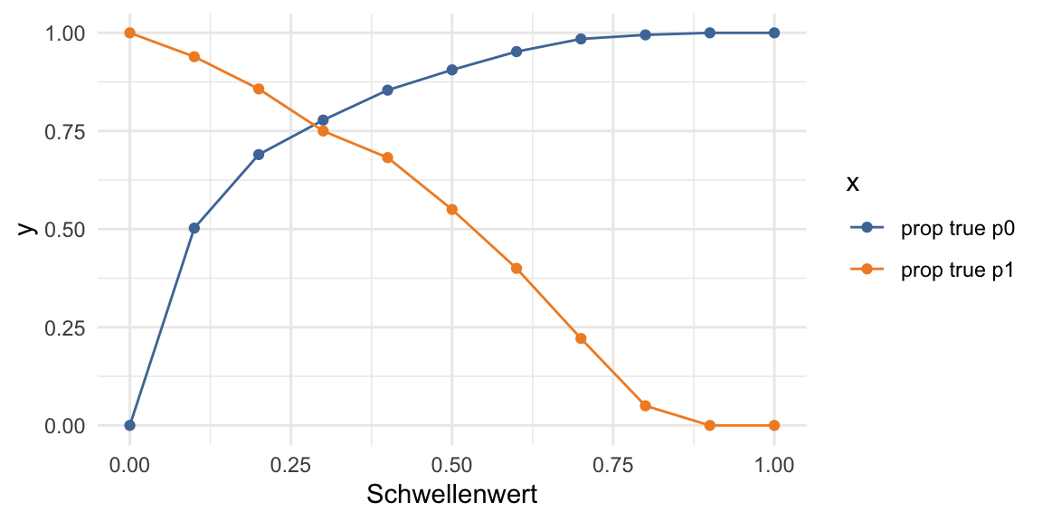
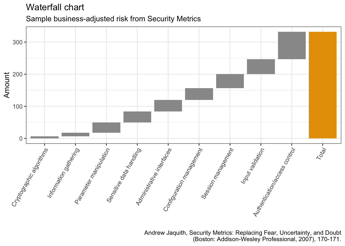
Below you’ll find the complete code and resources used to create the graphs in my talk The Good, the Bad and the Ugly: how to visualize Machine Learning data at this year’s Minds Mastering machines conference. You can find the German slides here:
You can find Part 1: The Good, the Bad and the Ugly: how (not) to visualize data here.
If you have questions or would like to talk about this article (or something else data-related), you can now book 15-minute timeslots with me (it’s free - one slot available per weekday):
This is an UPDATE to this old post with updated links & descriptions
This is code that accompanies a book chapter on customer churn that I have written for the German dpunkt Verlag. The book is in German, however.
The code you find below can be used to recreate all figures and analyses from this book chapter. Because the content is exclusively for the book, my descriptions around the code had to be minimal.
Editor’s note: This is a guest post by Nathaniel Schmucker. He is the founder of The Analyst Code, a blog that provides tools to instill a love of data in individuals of all backgrounds and to empower aspiring analysts.
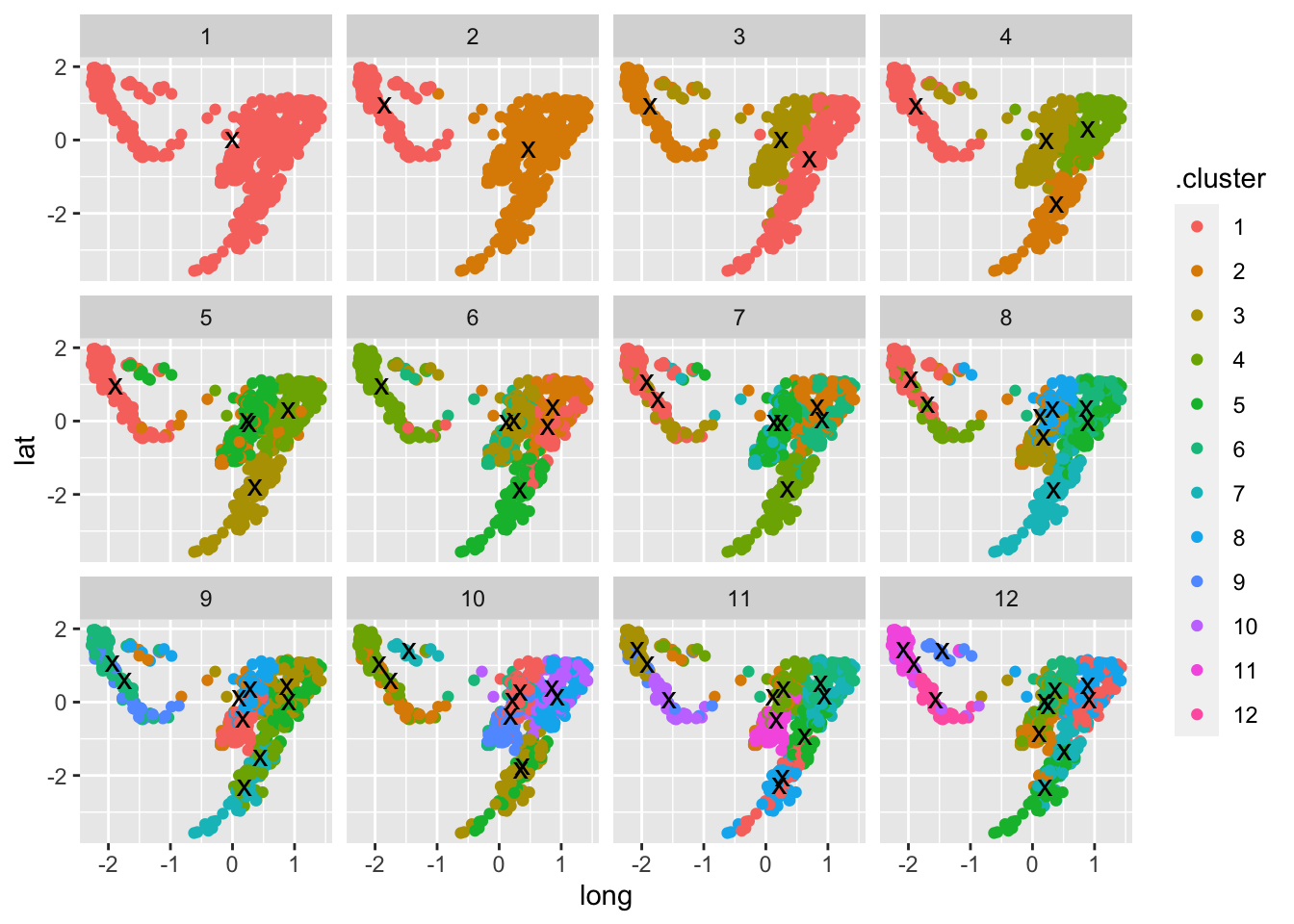
Introduction In this post, we will look at:
What is a k-Means analysis? How does the k-Means algorithm work? How do we implement k-Means in R?
Below you’ll find the complete code used to create the ggplot2 graphs in my talk The Good, the Bad and the Ugly: how (not) to visualize data at this year’s data2day conference. You can find the German slides here:
You can also find a German blog article accompanying my talk on codecentric’s blog.
If you have questions or would like to talk about this article (or something else data-related), you can now book 15-minute timeslots with me (it’s free - one slot available per weekday):