The Good, the Bad and the Ugly: how to visualize Machine Learning data
Below you’ll find the complete code and resources used to create the graphs in my talk The Good, the Bad and the Ugly: how to visualize Machine Learning data at this year’s Minds Mastering machines conference. You can find the German slides here:
You can find Part 1: The Good, the Bad and the Ugly: how (not) to visualize data here.
If you have questions or would like to talk about this article (or something else data-related), you can now book 15-minute timeslots with me (it’s free - one slot available per weekday):

If you have been enjoying my content and would like to help me be able to create more, please consider sending me a donation at . Thank you! :-)
Libraries
library(tidyverse)
library(mlbench)
library(ggfortify)
library(GGally)
library(scagnostics)
library(mlr)
Dataset
Pima Indians Diabetes dataset from mlbench package.
data(PimaIndiansDiabetes)
PimaIndiansDiabetes %>%
  head()
## pregnant glucose pressure triceps insulin mass pedigree age diabetes
## 1 6 148 72 35 0 33.6 0.627 50 pos
## 2 1 85 66 29 0 26.6 0.351 31 neg
## 3 8 183 64 0 0 23.3 0.672 32 pos
## 4 1 89 66 23 94 28.1 0.167 21 neg
## 5 0 137 40 35 168 43.1 2.288 33 pos
## 6 5 116 74 0 0 25.6 0.201 30 negColors
# The palette with grey:
cbp1 <- c("#999999", "#E69F00", "#56B4E9", "#009E73",
          "#F0E442", "#0072B2", "#D55E00", "#CC79A7")
ggplot <- function(...) ggplot2::ggplot(...) +
scale_color_manual(values = cbp1) +
scale_fill_manual(values = cbp1) + # note: needs to be overridden when using continuous color scales
theme_bw()Visualizing Machine Learning models
Visualizing different steps of the machine learning pipeline can help us
- explore the data (EDA),
- understand the data (and identify potential problems),
- pre-process the data in a suitable way for optimal model performance,
- supervise the learning process,
- optimize modeling,
- interpret the model and
- compare and evaluate model predictions.
Visualization also greatly simplifies communication of our model and results to decision-makers or the public.
Exploratory Data Analysis
Exploratory Data Analysis (EDA) is the backbone of data analysis, including those that result in a machine learning model. EDA helps us to understand the data we are working with and put it into context, so that we are able to ask the right questions (or to put our questions into the right frame). It also helps us take appropriate measures for cleaning, normalization/transformation, dealing with missing values, feature preparation and engineering, etc. Particularly if our machine learning model is trained on a limited dataset (but not only then!), appropriate data preparation can vastly improve the machine learning process: models will often train faster and achieve higher accuracy.
An essential part of EDA is data visualization.
Typically, we want to start by exploring potential sources of errors in our data, like
- wrong/useless data types (sometimes data types are automatically set in a way that is not useful for our analysis, like factors versus strings, or wrong/strange entries in an otherwise numeric column will make it categorical)
- missing values (a collection of ways to visualize missingness can be found here),
- outliers (for example by plotting a box-plot of continuous variables)
Depending on the number of features/variables we have, it makes sense to look at them all individually and in correlation with each other. Depending on whether we have a categorical or continuous variable, we might be interested in properties that are shown by
- histograms (frequency distribution of binned continuous variables),
- density distribution (normalized distribution of continuous variables) or
- bar-plots (shows counts of categorical variables).
If our target variable is categorical, we will want to look at potential imbalances between the classes. Class imbalance will strongly affect the machine learning modeling process and will require us to consider up-/downsampling or similar techniques before we train a model.
Correlation analysis can show us, for example
- how our target/dependent variable correlates with the remaining features (often, just by looking at the correlation, we can identify one ore more feature that will have a strong impact on predicting the target because they are strongly correlated) or
- whether some of the independent variables/features correlate with each other (multicolinearity; we might want to consider removing strongly correlated features, so that they won’t contribute the “same” information multiple times to the model and thus lead to overfitting).
Additional methods can be used to visualize groups of related features. These methods are often especially useful if we have a large dataset with a large feature set (highly dimensional data). Some of these methods for visualizing groups of related features and/or for comparing multiple variables and visualizing their relationships are:
- Dimensionality reduction:
- Principal Component Analysis (PCA, linear, shows as much variation in data as possible)
- Multidimensional scaling (MDS, non-linear)
- Sammon mapping (non-linear)
- T-Distributed Stochastic Neighbor Embedding (t-SNE, non-linear)
- Uniform Manifold Approximation and Projection (UMAP, non-linear, faster than T-SNE, often captures global variation better than T-SNE and PCA)
- Isometric Feature Mapping Ordination (Isomap)
- Parallel coordinate plots
- scagnostics
# in our dataset,
# continuous variables are
PimaIndiansDiabetes %>%
  dplyr::select(where(is.numeric)) %>%
  head()
## pregnant glucose pressure triceps insulin mass pedigree age
## 1 6 148 72 35 0 33.6 0.627 50
## 2 1 85 66 29 0 26.6 0.351 31
## 3 8 183 64 0 0 23.3 0.672 32
## 4 1 89 66 23 94 28.1 0.167 21
## 5 0 137 40 35 168 43.1 2.288 33
## 6 5 116 74 0 0 25.6 0.201 30# 'diabetes' is the only categorical variable is also our target or dependent variable
PimaIndiansDiabetes %>%
dplyr::select(!where(is.numeric)) %>%
head()## diabetes
## 1 pos
## 2 neg
## 3 pos
## 4 neg
## 5 pos
## 6 neg# bar plot of target
PimaIndiansDiabetes %>%
ggplot(aes(x = diabetes, fill = diabetes)) +
geom_bar(alpha = 0.8) +
theme(legend.position = "none") +
labs(x = "Diabetes outcome",
y = "count",
title = "Barplot of categorical features",
caption = "Source: Pima Indians Diabetes Database")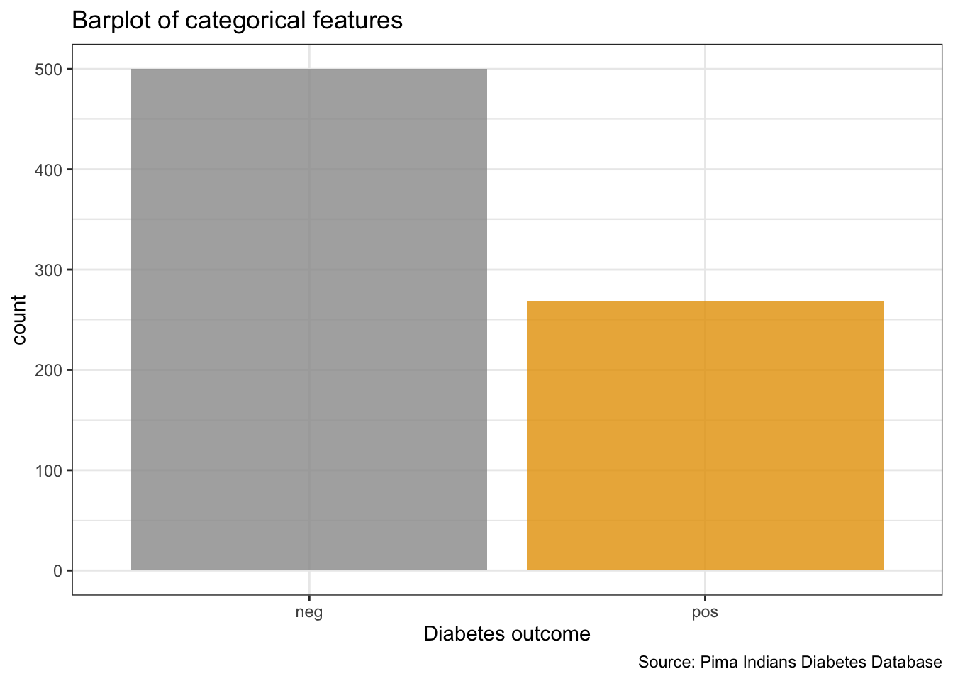
# boxplot of continuous features
PimaIndiansDiabetes %>%
  gather("key", "value", pregnant:age) %>%
  ggplot(aes(x = value, fill = diabetes)) +
    facet_wrap(vars(key), ncol = 3, scales = "free") +
    geom_boxplot(alpha = 0.8) +
    theme(axis.text.y = element_blank(),
          axis.ticks.y = element_blank())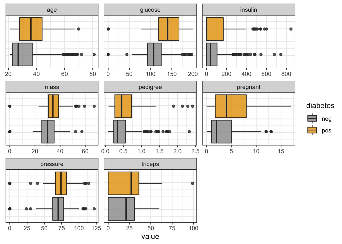
# histogram of features
PimaIndiansDiabetes %>%
  gather("key", "value", pregnant:age) %>%
  ggplot(aes(x = value, fill = diabetes)) +
    facet_wrap(vars(key), ncol = 3, scales = "free") +
    geom_histogram(alpha = 0.8) +
    labs(x = "value of feature in facet",
         y = "count",
         fill = "Diabetes",
        title = "Histogram of features",
        caption = "Source: Pima Indians Diabetes Database")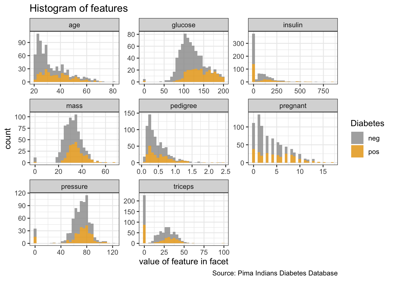
# density plot of of features
PimaIndiansDiabetes %>%
  gather("key", "value", pregnant:age) %>%
  ggplot(aes(x = value, fill = diabetes)) +
    facet_wrap(vars(key), ncol = 3, scales = "free") +
    geom_density(alpha = 0.8) +
    labs(x = "value of feature in facet",
         y = "density",
         fill = "Diabetes",
        title = "Density of continuous features",
        caption = "Source: Pima Indians Diabetes Database")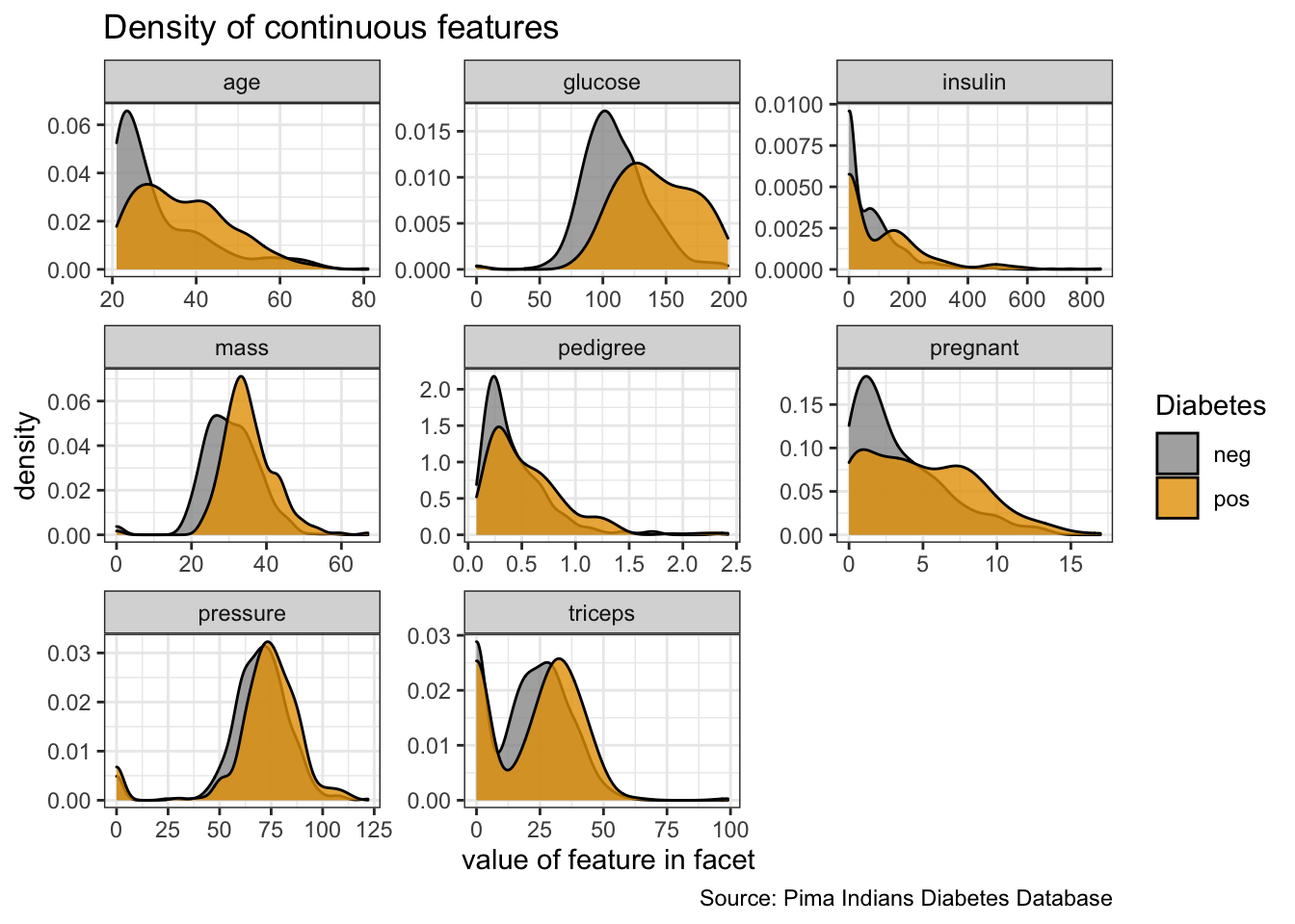
# correlation plot of features
mat <- PimaIndiansDiabetes %>%
  dplyr::select(where(is.numeric))

cormat <- round(cor(mat), 2)

cormat <- cormat %>%
  as_data_frame() %>%
  mutate(x = colnames(mat)) %>%
  gather(key = "y", value = "value", pregnant:age)

cormat %>%
    remove_missing() %>%
    arrange(x, y) %>%
    ggplot(aes(x = x, y = y, fill = value)) +
    geom_tile() +
    scale_fill_gradient2(low = "blue", high = "red", mid = "white",
     midpoint = 0, limit = c(-1,1), space = "Lab",
     name = "Pearson\nCorrelation") +
    theme(axis.text.x = element_text(angle = 45, vjust = 1, hjust = 1)) +
    coord_fixed() +
    labs(x = "feature",
         y = "feature",
        title = "Correlation between features",
        caption = "Source: Pima Indians Diabetes Database")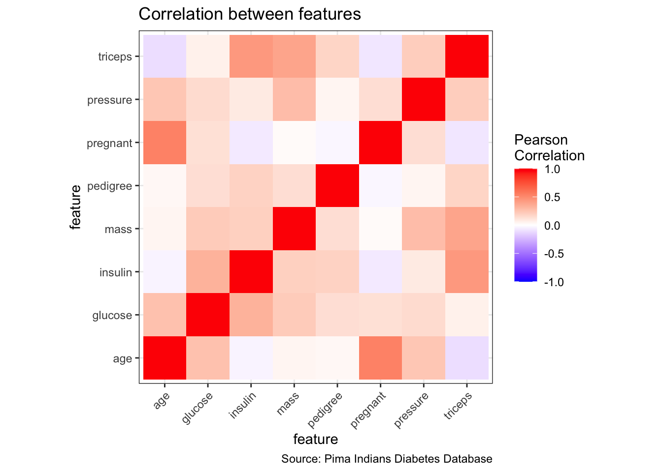
# scatterplot matrix
ggpairs(PimaIndiansDiabetes,
        columns = c(1:8),
        alpha = 0.7) +
    labs(x = "feature",
         y = "feature",
        title = "Scatterplot matrix",
        caption = "Source: Pima Indians Diabetes Database")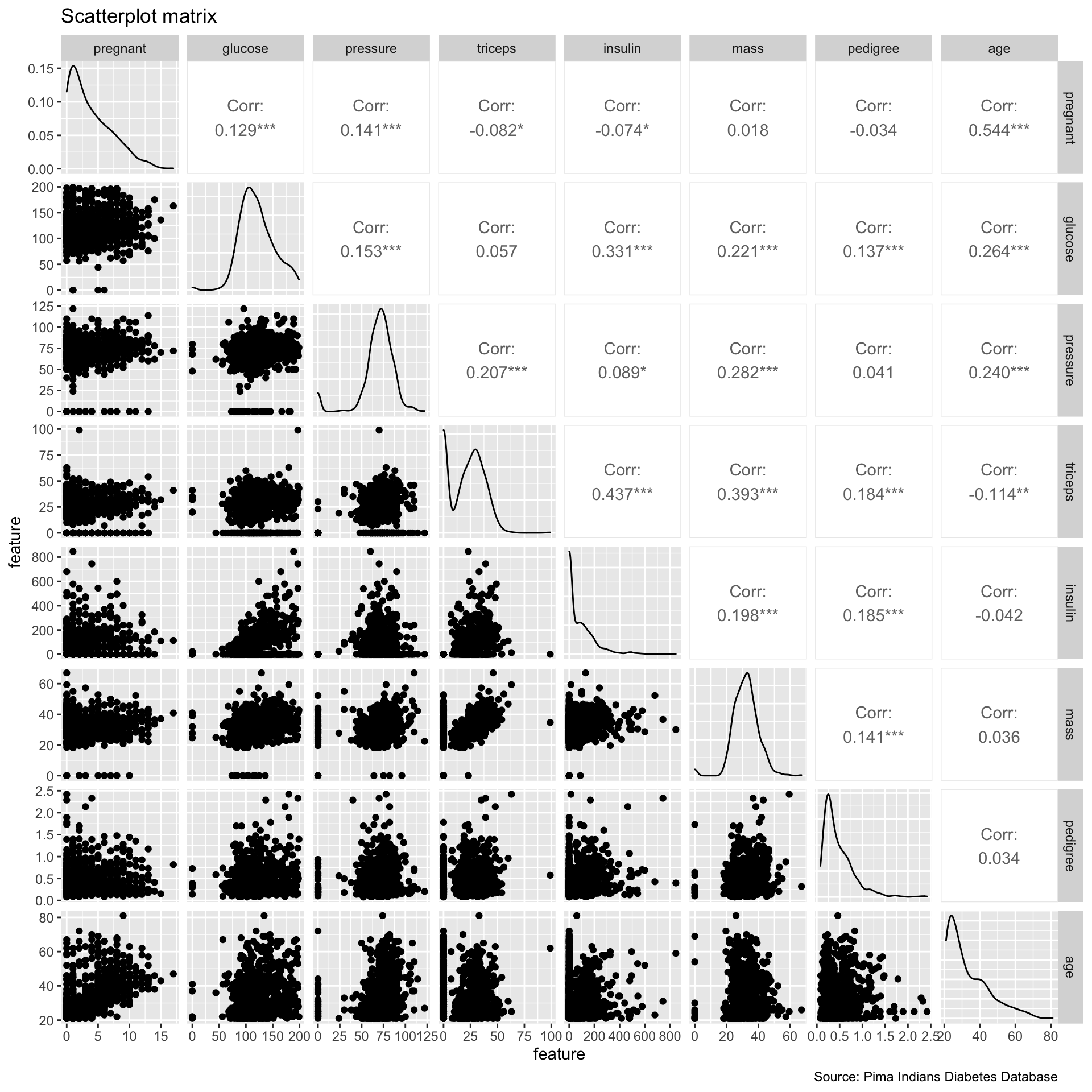
# PCA
prep <- PimaIndiansDiabetes %>%
  dplyr::select(where(is.numeric))

pca <- prep %>%
  prcomp(scale. = TRUE)

autoplot(pca,
                data = PimaIndiansDiabetes,
                colour = 'diabetes',
                shape = 'diabetes',
                loadings = TRUE,
                loadings.colour = 'blue',
                loadings.label = TRUE,
                loadings.label.size = 3) +
      scale_color_manual(values = cbp1) +
  scale_fill_manual(values = cbp1) +
  theme_bw() +
    labs(title = "Principal Component Analysis (PCA)",
        caption = "Source: Pima Indians Diabetes Database")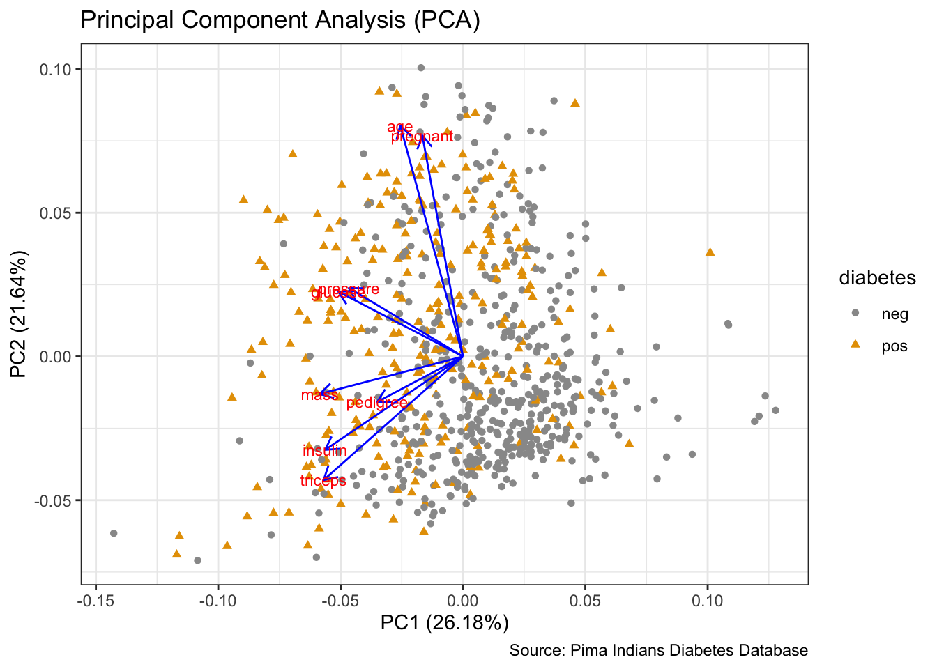
# MDS
d <- dist(prep) # euclidean distances between the rows
fit <- cmdscale(d,eig=TRUE, k=2) # k is the number of dim
fit$points %>%
  head()
## [,1] [,2]
## 1 -75.71465 -35.950783
## 2 -82.35827 28.908213
## 3 -74.63064 -67.906496
## 4 11.07742 34.898486
## 5 89.74379 -2.746937
## 6 -80.97792 -3.946887# Sammon mapping
library(MASS)
sam <- sammon(dist(prep))## Initial stress : 0.03033
## stress after 0 iters: 0.03033sam$points %>%
head()## [,1] [,2]
## 1 -75.71465 -35.950783
## 2 -82.35827 28.908213
## 3 -74.63064 -67.906496
## 4 11.07742 34.898486
## 5 89.74379 -2.746937
## 6 -80.97792 -3.946887# parallel coordinate plots
ggparcoord(data = PimaIndiansDiabetes,
columns = c(1:8),
groupColumn = 9,
scale = "robust",
order = "skewness",
alpha = 0.7)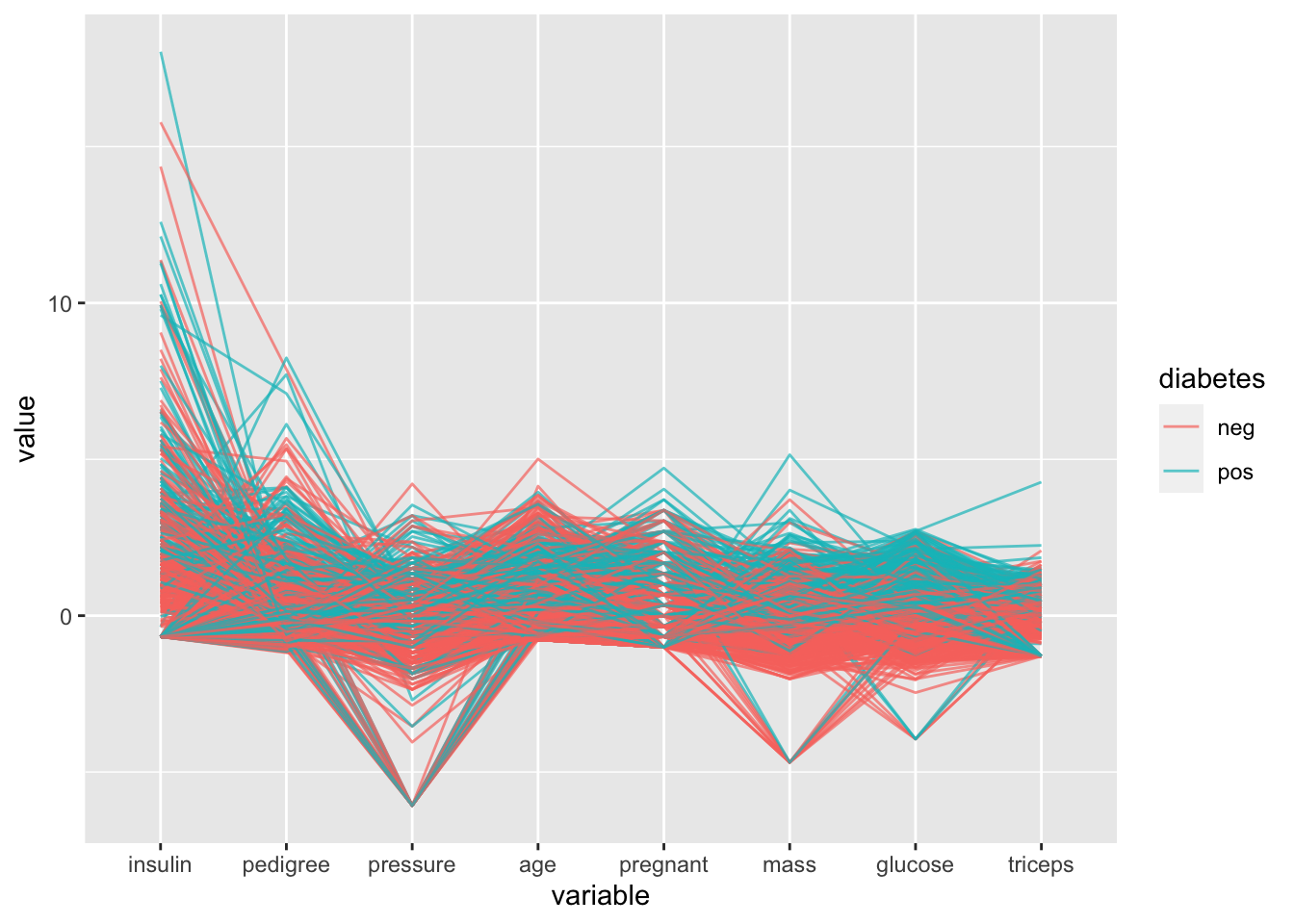
# scagnostics
scagnostics_dataset <- scagnostics(PimaIndiansDiabetes)

# scagnostics grid
scagnostics_grid_dataset <- scagnosticsGrid(scagnostics_dataset)

# outliers
scagnostics_o_dataset <- scagnosticsOutliers(scagnostics_dataset)
scagnostics_o_dataset[scagnostics_o_dataset]
## pregnant * age
## TRUEoutlier <- scagnostics_grid_dataset[scagnostics_o_dataset,]
# scagnostics exemplars
scagnostics_ex_dataset <- scagnosticsExemplars(scagnostics_dataset)
scagnostics_ex_dataset[scagnostics_ex_dataset]## pregnant * triceps mass * age triceps * diabetes
## TRUE TRUE TRUEexemplars <- scagnostics_grid_dataset[scagnostics_ex_dataset,]Training a machine learning model
(using mlr package)
- create training and test set
set.seed(1000)

train_index <- sample(1:nrow(PimaIndiansDiabetes), 0.8 * nrow(PimaIndiansDiabetes))
test_index <- setdiff(1:nrow(PimaIndiansDiabetes), train_index)

train <- PimaIndiansDiabetes[train_index,]
test <- PimaIndiansDiabetes[test_index,]

list( train = summary(train), test = summary(test) )
## $train
## pregnant glucose pressure triceps
## Min. : 0.000 Min. : 0.0 Min. : 0.00 Min. : 0.00
## 1st Qu.: 1.000 1st Qu.:100.0 1st Qu.: 64.00 1st Qu.: 0.00
## Median : 3.000 Median :119.0 Median : 72.00 Median :23.00
## Mean : 3.894 Mean :123.1 Mean : 68.89 Mean :20.66
## 3rd Qu.: 6.000 3rd Qu.:143.0 3rd Qu.: 80.00 3rd Qu.:32.75
## Max. :17.000 Max. :199.0 Max. :114.00 Max. :99.00
## insulin mass pedigree age diabetes
## Min. : 0.00 Min. : 0.00 Min. :0.0780 Min. :21.00 neg:386
## 1st Qu.: 0.00 1st Qu.:27.10 1st Qu.:0.2442 1st Qu.:24.00 pos:228
## Median : 36.50 Median :32.00 Median :0.3780 Median :29.00
## Mean : 81.65 Mean :31.92 Mean :0.4742 Mean :33.42
## 3rd Qu.:131.50 3rd Qu.:36.38 3rd Qu.:0.6355 3rd Qu.:41.00
## Max. :846.00 Max. :59.40 Max. :2.4200 Max. :81.00
##
## $test
## pregnant glucose pressure triceps
## Min. : 0.000 Min. : 0.0 Min. : 0.00 Min. : 0.00
## 1st Qu.: 1.000 1st Qu.: 93.0 1st Qu.: 62.00 1st Qu.: 0.00
## Median : 2.000 Median :108.0 Median : 72.00 Median :23.00
## Mean : 3.649 Mean :112.3 Mean : 69.96 Mean :20.03
## 3rd Qu.: 6.000 3rd Qu.:133.8 3rd Qu.: 79.50 3rd Qu.:32.00
## Max. :14.000 Max. :197.0 Max. :122.00 Max. :56.00
## insulin mass pedigree age diabetes
## Min. : 0.0 Min. : 0.00 Min. :0.0850 Min. :21.00 neg:114
## 1st Qu.: 0.0 1st Qu.:27.80 1st Qu.:0.2395 1st Qu.:23.25 pos: 40
## Median : 20.5 Median :32.40 Median :0.3380 Median :29.00
## Mean : 72.4 Mean :32.29 Mean :0.4627 Mean :32.54
## 3rd Qu.:100.0 3rd Qu.:36.88 3rd Qu.:0.6008 3rd Qu.:39.75
## Max. :744.0 Max. :67.10 Max. :2.3290 Max. :67.00- create classification task and learner
listLearners() %>%
  head()
## class name short.name
## 1 classif.ada ada Boosting ada
## 2 classif.adaboostm1 ada Boosting M1 adaboostm1
## 3 classif.bartMachine Bayesian Additive Regression Trees bartmachine
## 4 classif.binomial Binomial Regression binomial
## 5 classif.boosting Adabag Boosting adabag
## 6 classif.bst Gradient Boosting bst
## package
## 1 ada,rpart
## 2 RWeka
## 3 bartMachine
## 4 stats
## 5 adabag,rpart
## 6 bst,rpart
## note
## 1 `xval` has been set to `0` by default for speed.
## 2 NAs are directly passed to WEKA with `na.action = na.pass`.
## 3 `use_missing_data` has been set to `TRUE` by default to allow missing data support.
## 4 Delegates to `glm` with freely choosable binomial link function via learner parameter `link`. We set 'model' to FALSE by default to save memory.
## 5 `xval` has been set to `0` by default for speed.
## 6 Renamed parameter `learner` to `Learner` due to nameclash with `setHyperPars`. Default changes: `Learner = "ls"`, `xval = 0`, and `maxdepth = 1`.
## type installed numerics factors ordered missings weights prob oneclass
## 1 classif FALSE TRUE TRUE FALSE FALSE FALSE TRUE FALSE
## 2 classif TRUE TRUE TRUE FALSE FALSE FALSE TRUE FALSE
## 3 classif FALSE TRUE TRUE FALSE TRUE FALSE TRUE FALSE
## 4 classif TRUE TRUE TRUE FALSE FALSE TRUE TRUE FALSE
## 5 classif FALSE TRUE TRUE FALSE TRUE FALSE TRUE FALSE
## 6 classif FALSE TRUE FALSE FALSE FALSE FALSE FALSE FALSE
## twoclass multiclass class.weights featimp oobpreds functionals
## 1 TRUE FALSE FALSE FALSE FALSE FALSE
## 2 TRUE TRUE FALSE FALSE FALSE FALSE
## 3 TRUE FALSE FALSE FALSE FALSE FALSE
## 4 TRUE FALSE FALSE FALSE FALSE FALSE
## 5 TRUE TRUE FALSE TRUE FALSE FALSE
## 6 TRUE FALSE FALSE FALSE FALSE FALSE
## single.functional se lcens rcens icens
## 1 FALSE FALSE FALSE FALSE FALSE
## 2 FALSE FALSE FALSE FALSE FALSE
## 3 FALSE FALSE FALSE FALSE FALSE
## 4 FALSE FALSE FALSE FALSE FALSE
## 5 FALSE FALSE FALSE FALSE FALSE
## 6 FALSE FALSE FALSE FALSE FALSE(dt_task <- makeClassifTask(data = train, target = "diabetes"))## Supervised task: train
## Type: classif
## Target: diabetes
## Observations: 614
## Features:
## numerics factors ordered functionals
## 8 0 0 0
## Missings: FALSE
## Has weights: FALSE
## Has blocking: FALSE
## Has coordinates: FALSE
## Classes: 2
## neg pos
## 386 228
## Positive class: neg(dt_prob <- makeLearner('classif.gbm', predict.type = "prob"))## Learner classif.gbm from package gbm
## Type: classif
## Name: Gradient Boosting Machine; Short name: gbm
## Class: classif.gbm
## Properties: twoclass,multiclass,missings,numerics,factors,prob,weights,featimp
## Predict-Type: prob
## Hyperparameters: keep.data=FALSEFeature Selection
library(FSelector)

listFilterMethods() %>%
  head()
## id package desc
## 1 anova.test ANOVA Test for binary and multiclass ...
## 2 auc AUC filter for binary classification ...
## 3 carscore care CAR scores
## 4 FSelector_chi.squared FSelector Chi-squared statistic of independence...
## 5 FSelector_gain.ratio FSelector Chi-squared statistic of independence...
## 6 FSelector_information.gain FSelector Entropy-based information gain betwee...listFilterEnsembleMethods() %>%
head()## id
## 1 E-Borda
## 2 E-max
## 3 E-mean
## 4 E-median
## 5 E-min
## desc
## 1 Borda ensemble filter. Takes the sum across all base filter methods for each feature.
## 2 Maximum ensemble filter. Takes the best maximum value across all base filter methods for each feature.
## 3 Mean ensemble filter. Takes the mean across all base filter methods for each feature.
## 4 Median ensemble filter. Takes the median across all base filter methods for each feature.
## 5 Minimum ensemble filter. Takes the best minimum value across all base filter methods for each feature.generateFilterValuesData(dt_task, method = "FSelector_information.gain") %>%
plotFilterValues() +
theme_bw() +
labs(x = "feature",
y = "information gain",
title = "Information gain of features in GBM",
caption = "Source: Pima Indians Diabetes Database")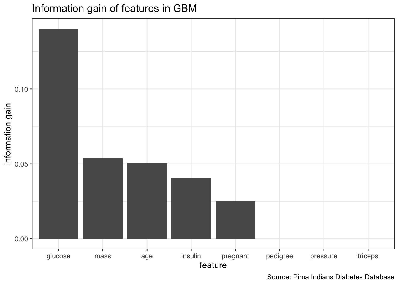
feat_imp_tpr <- generateFeatureImportanceData(task = dt_task,
                              learner = dt_prob,
                              measure = tpr,
                              interaction = FALSE)
## Distribution not specified, assuming bernoulli ...feat_imp_tpr$res %>%
gather() %>%
ggplot(aes(x = reorder(key, value), y = value)) +
geom_bar(stat = "identity") +
labs(x = "feature",
title = "True positive rate of features in GBM",
subtitle = "calculated with permutation importance",
caption = "Source: Pima Indians Diabetes Database")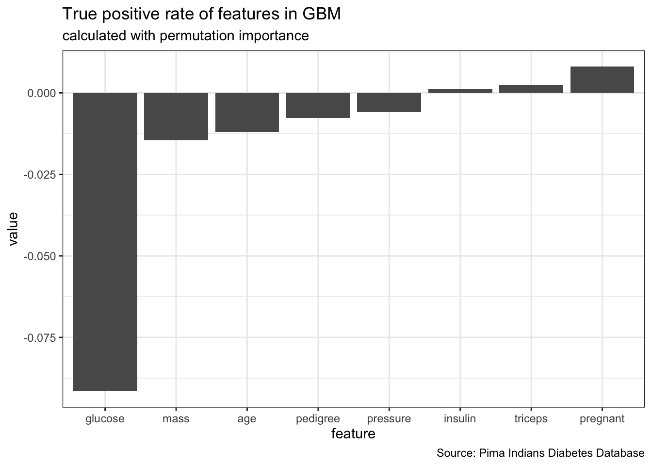
feat_imp_auc <- generateFeatureImportanceData(task = dt_task,
                              learner = dt_prob,
                              measure = auc,
                              interaction = FALSE)
## Distribution not specified, assuming bernoulli ...feat_imp_auc$res %>%
gather() %>%
ggplot(aes(x = reorder(key, value), y = value)) +
geom_bar(stat = "identity") +
labs(x = "feature",
title = "Area under the curve of features in GBM",
subtitle = "calculated with permutation importance",
caption = "Source: Pima Indians Diabetes Database")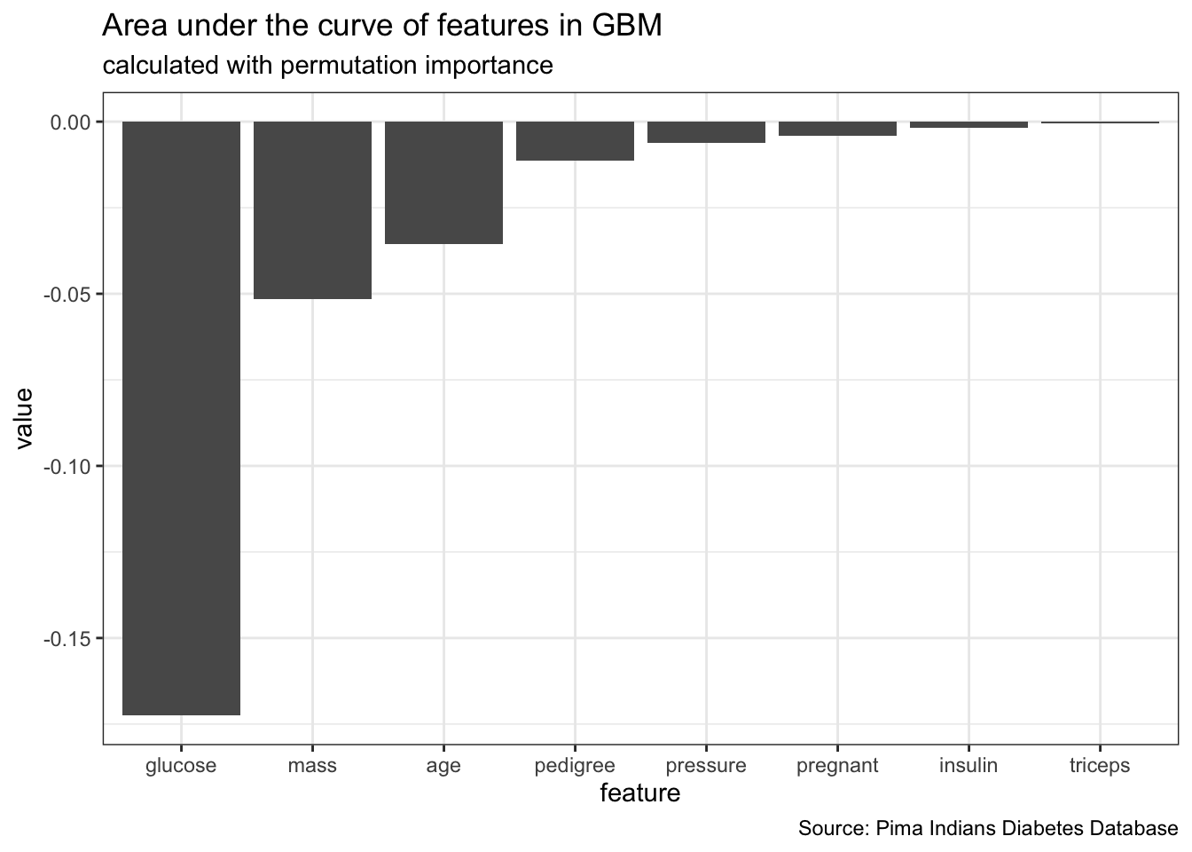
set.seed(1000)
train <- dplyr::select(train, -pedigree, -pressure, -triceps)
test <- dplyr::select(test, -pedigree, -pressure, -triceps)
list(train = summary(train), test = summary(test))
## $train
## pregnant glucose insulin mass
## Min. : 0.000 Min. : 0.0 Min. : 0.00 Min. : 0.00
## 1st Qu.: 1.000 1st Qu.:100.0 1st Qu.: 0.00 1st Qu.:27.10
## Median : 3.000 Median :119.0 Median : 36.50 Median :32.00
## Mean : 3.894 Mean :123.1 Mean : 81.65 Mean :31.92
## 3rd Qu.: 6.000 3rd Qu.:143.0 3rd Qu.:131.50 3rd Qu.:36.38
## Max. :17.000 Max. :199.0 Max. :846.00 Max. :59.40
## age diabetes
## Min. :21.00 neg:386
## 1st Qu.:24.00 pos:228
## Median :29.00
## Mean :33.42
## 3rd Qu.:41.00
## Max. :81.00
##
## $test
## pregnant glucose insulin mass
## Min. : 0.000 Min. : 0.0 Min. : 0.0 Min. : 0.00
## 1st Qu.: 1.000 1st Qu.: 93.0 1st Qu.: 0.0 1st Qu.:27.80
## Median : 2.000 Median :108.0 Median : 20.5 Median :32.40
## Mean : 3.649 Mean :112.3 Mean : 72.4 Mean :32.29
## 3rd Qu.: 6.000 3rd Qu.:133.8 3rd Qu.:100.0 3rd Qu.:36.88
## Max. :14.000 Max. :197.0 Max. :744.0 Max. :67.10
## age diabetes
## Min. :21.00 neg:114
## 1st Qu.:23.25 pos: 40
## Median :29.00
## Mean :32.54
## 3rd Qu.:39.75
## Max. :67.00(dt_task <- makeClassifTask(data = train, target = "diabetes"))## Supervised task: train
## Type: classif
## Target: diabetes
## Observations: 614
## Features:
## numerics factors ordered functionals
## 5 0 0 0
## Missings: FALSE
## Has weights: FALSE
## Has blocking: FALSE
## Has coordinates: FALSE
## Classes: 2
## neg pos
## 386 228
## Positive class: negHyperparameter Optimization
getParamSet("classif.gbm")## Type len Def
## distribution discrete - bernoulli
## n.trees integer - 100
## cv.folds integer - 0
## interaction.depth integer - 1
## n.minobsinnode integer - 10
## shrinkage numeric - 0.1
## bag.fraction numeric - 0.5
## train.fraction numeric - 1
## keep.data logical - TRUE
## verbose logical - FALSE
## n.cores integer - 1
## Constr Req Tunable Trafo
## distribution gaussian,bernoulli,huberized,adaboost... - TRUE -
## n.trees 1 to Inf - TRUE -
## cv.folds -Inf to Inf - TRUE -
## interaction.depth 1 to Inf - TRUE -
## n.minobsinnode 1 to Inf - TRUE -
## shrinkage 0 to Inf - TRUE -
## bag.fraction 0 to 1 - TRUE -
## train.fraction 0 to 1 - TRUE -
## keep.data - - FALSE -
## verbose - - FALSE -
## n.cores -Inf to Inf - FALSE -dt_param <- makeParamSet(
makeIntegerParam("n.trees", lower = 20, upper = 150),
makeNumericParam("shrinkage", lower = 0.01, upper = 0.1))
ctrl = makeTuneControlGrid()
rdesc = makeResampleDesc("CV",
iters = 3L,
stratify = TRUE)set.seed(1000)
(dt_tuneparam <- tuneParams(learner = dt_prob,
resampling = rdesc,
measures = list(tpr,auc, fnr, mmce, tnr, setAggregation(tpr, test.sd)),
par.set = dt_param,
control = ctrl,
task = dt_task,
show.info = FALSE))## Distribution not specified, assuming bernoulli ...
## Distribution not specified, assuming bernoulli ...
## Distribution not specified, assuming bernoulli ...
## Distribution not specified, assuming bernoulli ...
## Distribution not specified, assuming bernoulli ...
## Distribution not specified, assuming bernoulli ...
## Distribution not specified, assuming bernoulli ...
## Distribution not specified, assuming bernoulli ...
## Distribution not specified, assuming bernoulli ...
## Distribution not specified, assuming bernoulli ...
## Distribution not specified, assuming bernoulli ...
## Distribution not specified, assuming bernoulli ...
## Distribution not specified, assuming bernoulli ...
## Distribution not specified, assuming bernoulli ...
## Distribution not specified, assuming bernoulli ...
## Distribution not specified, assuming bernoulli ...
## Distribution not specified, assuming bernoulli ...
## Distribution not specified, assuming bernoulli ...
## Distribution not specified, assuming bernoulli ...
## Distribution not specified, assuming bernoulli ...
## Distribution not specified, assuming bernoulli ...
## Distribution not specified, assuming bernoulli ...
## Distribution not specified, assuming bernoulli ...
## Distribution not specified, assuming bernoulli ...
## Distribution not specified, assuming bernoulli ...
## Distribution not specified, assuming bernoulli ...
## Distribution not specified, assuming bernoulli ...
## Distribution not specified, assuming bernoulli ...
## Distribution not specified, assuming bernoulli ...
## Distribution not specified, assuming bernoulli ...
## Distribution not specified, assuming bernoulli ...
## Distribution not specified, assuming bernoulli ...
## Distribution not specified, assuming bernoulli ...
## Distribution not specified, assuming bernoulli ...
## Distribution not specified, assuming bernoulli ...
## Distribution not specified, assuming bernoulli ...
## Distribution not specified, assuming bernoulli ...
## Distribution not specified, assuming bernoulli ...
## Distribution not specified, assuming bernoulli ...
## Distribution not specified, assuming bernoulli ...
## Distribution not specified, assuming bernoulli ...
## Distribution not specified, assuming bernoulli ...
## Distribution not specified, assuming bernoulli ...
## Distribution not specified, assuming bernoulli ...
## Distribution not specified, assuming bernoulli ...
## Distribution not specified, assuming bernoulli ...
## Distribution not specified, assuming bernoulli ...
## Distribution not specified, assuming bernoulli ...
## Distribution not specified, assuming bernoulli ...
## Distribution not specified, assuming bernoulli ...
## Distribution not specified, assuming bernoulli ...
## Distribution not specified, assuming bernoulli ...
## Distribution not specified, assuming bernoulli ...
## Distribution not specified, assuming bernoulli ...
## Distribution not specified, assuming bernoulli ...
## Distribution not specified, assuming bernoulli ...
## Distribution not specified, assuming bernoulli ...
## Distribution not specified, assuming bernoulli ...
## Distribution not specified, assuming bernoulli ...
## Distribution not specified, assuming bernoulli ...
## Distribution not specified, assuming bernoulli ...
## Distribution not specified, assuming bernoulli ...
## Distribution not specified, assuming bernoulli ...
## Distribution not specified, assuming bernoulli ...
## Distribution not specified, assuming bernoulli ...
## Distribution not specified, assuming bernoulli ...
## Distribution not specified, assuming bernoulli ...
## Distribution not specified, assuming bernoulli ...
## Distribution not specified, assuming bernoulli ...
## Distribution not specified, assuming bernoulli ...
## Distribution not specified, assuming bernoulli ...
## Distribution not specified, assuming bernoulli ...
## Distribution not specified, assuming bernoulli ...
## Distribution not specified, assuming bernoulli ...
## Distribution not specified, assuming bernoulli ...
## Distribution not specified, assuming bernoulli ...
## Distribution not specified, assuming bernoulli ...
## Distribution not specified, assuming bernoulli ...
## Distribution not specified, assuming bernoulli ...
## Distribution not specified, assuming bernoulli ...
## Distribution not specified, assuming bernoulli ...
## Distribution not specified, assuming bernoulli ...
## Distribution not specified, assuming bernoulli ...
## Distribution not specified, assuming bernoulli ...
## Distribution not specified, assuming bernoulli ...
## Distribution not specified, assuming bernoulli ...
## Distribution not specified, assuming bernoulli ...
## Distribution not specified, assuming bernoulli ...
## Distribution not specified, assuming bernoulli ...
## Distribution not specified, assuming bernoulli ...
## Distribution not specified, assuming bernoulli ...
## Distribution not specified, assuming bernoulli ...
## Distribution not specified, assuming bernoulli ...
## Distribution not specified, assuming bernoulli ...
## Distribution not specified, assuming bernoulli ...
## Distribution not specified, assuming bernoulli ...
## Distribution not specified, assuming bernoulli ...
## Distribution not specified, assuming bernoulli ...
## Distribution not specified, assuming bernoulli ...
## Distribution not specified, assuming bernoulli ...
## Distribution not specified, assuming bernoulli ...
## Distribution not specified, assuming bernoulli ...
## Distribution not specified, assuming bernoulli ...
## Distribution not specified, assuming bernoulli ...
## Distribution not specified, assuming bernoulli ...
## Distribution not specified, assuming bernoulli ...
## Distribution not specified, assuming bernoulli ...
## Distribution not specified, assuming bernoulli ...
## Distribution not specified, assuming bernoulli ...
## Distribution not specified, assuming bernoulli ...
## Distribution not specified, assuming bernoulli ...
## Distribution not specified, assuming bernoulli ...
## Distribution not specified, assuming bernoulli ...
## Distribution not specified, assuming bernoulli ...
## Distribution not specified, assuming bernoulli ...
## Distribution not specified, assuming bernoulli ...
## Distribution not specified, assuming bernoulli ...
## Distribution not specified, assuming bernoulli ...
## Distribution not specified, assuming bernoulli ...
## Distribution not specified, assuming bernoulli ...
## Distribution not specified, assuming bernoulli ...
## Distribution not specified, assuming bernoulli ...
## Distribution not specified, assuming bernoulli ...
## Distribution not specified, assuming bernoulli ...
## Distribution not specified, assuming bernoulli ...
## Distribution not specified, assuming bernoulli ...
## Distribution not specified, assuming bernoulli ...
## Distribution not specified, assuming bernoulli ...
## Distribution not specified, assuming bernoulli ...
## Distribution not specified, assuming bernoulli ...
## Distribution not specified, assuming bernoulli ...
## Distribution not specified, assuming bernoulli ...
## Distribution not specified, assuming bernoulli ...
## Distribution not specified, assuming bernoulli ...
## Distribution not specified, assuming bernoulli ...
## Distribution not specified, assuming bernoulli ...
## Distribution not specified, assuming bernoulli ...
## Distribution not specified, assuming bernoulli ...
## Distribution not specified, assuming bernoulli ...
## Distribution not specified, assuming bernoulli ...
## Distribution not specified, assuming bernoulli ...
## Distribution not specified, assuming bernoulli ...
## Distribution not specified, assuming bernoulli ...
## Distribution not specified, assuming bernoulli ...
## Distribution not specified, assuming bernoulli ...
## Distribution not specified, assuming bernoulli ...
## Distribution not specified, assuming bernoulli ...
## Distribution not specified, assuming bernoulli ...
## Distribution not specified, assuming bernoulli ...
## Distribution not specified, assuming bernoulli ...
## Distribution not specified, assuming bernoulli ...
## Distribution not specified, assuming bernoulli ...
## Distribution not specified, assuming bernoulli ...
## Distribution not specified, assuming bernoulli ...
## Distribution not specified, assuming bernoulli ...
## Distribution not specified, assuming bernoulli ...
## Distribution not specified, assuming bernoulli ...
## Distribution not specified, assuming bernoulli ...
## Distribution not specified, assuming bernoulli ...
## Distribution not specified, assuming bernoulli ...
## Distribution not specified, assuming bernoulli ...
## Distribution not specified, assuming bernoulli ...
## Distribution not specified, assuming bernoulli ...
## Distribution not specified, assuming bernoulli ...
## Distribution not specified, assuming bernoulli ...
## Distribution not specified, assuming bernoulli ...
## Distribution not specified, assuming bernoulli ...
## Distribution not specified, assuming bernoulli ...
## Distribution not specified, assuming bernoulli ...
## Distribution not specified, assuming bernoulli ...
## Distribution not specified, assuming bernoulli ...
## Distribution not specified, assuming bernoulli ...
## Distribution not specified, assuming bernoulli ...
## Distribution not specified, assuming bernoulli ...
## Distribution not specified, assuming bernoulli ...
## Distribution not specified, assuming bernoulli ...
## Distribution not specified, assuming bernoulli ...
## Distribution not specified, assuming bernoulli ...
## Distribution not specified, assuming bernoulli ...
## Distribution not specified, assuming bernoulli ...
## Distribution not specified, assuming bernoulli ...
## Distribution not specified, assuming bernoulli ...
## Distribution not specified, assuming bernoulli ...
## Distribution not specified, assuming bernoulli ...
## Distribution not specified, assuming bernoulli ...
## Distribution not specified, assuming bernoulli ...
## Distribution not specified, assuming bernoulli ...
## Distribution not specified, assuming bernoulli ...
## Distribution not specified, assuming bernoulli ...
## Distribution not specified, assuming bernoulli ...
## Distribution not specified, assuming bernoulli ...
## Distribution not specified, assuming bernoulli ...
## Distribution not specified, assuming bernoulli ...
## Distribution not specified, assuming bernoulli ...
## Distribution not specified, assuming bernoulli ...
## Distribution not specified, assuming bernoulli ...
## Distribution not specified, assuming bernoulli ...
## Distribution not specified, assuming bernoulli ...
## Distribution not specified, assuming bernoulli ...
## Distribution not specified, assuming bernoulli ...
## Distribution not specified, assuming bernoulli ...
## Distribution not specified, assuming bernoulli ...
## Distribution not specified, assuming bernoulli ...
## Distribution not specified, assuming bernoulli ...
## Distribution not specified, assuming bernoulli ...
## Distribution not specified, assuming bernoulli ...
## Distribution not specified, assuming bernoulli ...
## Distribution not specified, assuming bernoulli ...
## Distribution not specified, assuming bernoulli ...
## Distribution not specified, assuming bernoulli ...
## Distribution not specified, assuming bernoulli ...
## Distribution not specified, assuming bernoulli ...
## Distribution not specified, assuming bernoulli ...
## Distribution not specified, assuming bernoulli ...
## Distribution not specified, assuming bernoulli ...
## Distribution not specified, assuming bernoulli ...
## Distribution not specified, assuming bernoulli ...
## Distribution not specified, assuming bernoulli ...
## Distribution not specified, assuming bernoulli ...
## Distribution not specified, assuming bernoulli ...
## Distribution not specified, assuming bernoulli ...
## Distribution not specified, assuming bernoulli ...
## Distribution not specified, assuming bernoulli ...
## Distribution not specified, assuming bernoulli ...
## Distribution not specified, assuming bernoulli ...
## Distribution not specified, assuming bernoulli ...
## Distribution not specified, assuming bernoulli ...
## Distribution not specified, assuming bernoulli ...
## Distribution not specified, assuming bernoulli ...
## Distribution not specified, assuming bernoulli ...
## Distribution not specified, assuming bernoulli ...
## Distribution not specified, assuming bernoulli ...
## Distribution not specified, assuming bernoulli ...
## Distribution not specified, assuming bernoulli ...
## Distribution not specified, assuming bernoulli ...
## Distribution not specified, assuming bernoulli ...
## Distribution not specified, assuming bernoulli ...
## Distribution not specified, assuming bernoulli ...
## Distribution not specified, assuming bernoulli ...
## Distribution not specified, assuming bernoulli ...
## Distribution not specified, assuming bernoulli ...
## Distribution not specified, assuming bernoulli ...
## Distribution not specified, assuming bernoulli ...
## Distribution not specified, assuming bernoulli ...
## Distribution not specified, assuming bernoulli ...
## Distribution not specified, assuming bernoulli ...
## Distribution not specified, assuming bernoulli ...
## Distribution not specified, assuming bernoulli ...
## Distribution not specified, assuming bernoulli ...
## Distribution not specified, assuming bernoulli ...
## Distribution not specified, assuming bernoulli ...
## Distribution not specified, assuming bernoulli ...
## Distribution not specified, assuming bernoulli ...
## Distribution not specified, assuming bernoulli ...
## Distribution not specified, assuming bernoulli ...
## Distribution not specified, assuming bernoulli ...
## Distribution not specified, assuming bernoulli ...
## Distribution not specified, assuming bernoulli ...
## Distribution not specified, assuming bernoulli ...
## Distribution not specified, assuming bernoulli ...
## Distribution not specified, assuming bernoulli ...
## Distribution not specified, assuming bernoulli ...
## Distribution not specified, assuming bernoulli ...
## Distribution not specified, assuming bernoulli ...
## Distribution not specified, assuming bernoulli ...
## Distribution not specified, assuming bernoulli ...
## Distribution not specified, assuming bernoulli ...
## Distribution not specified, assuming bernoulli ...
## Distribution not specified, assuming bernoulli ...
## Distribution not specified, assuming bernoulli ...
## Distribution not specified, assuming bernoulli ...
## Distribution not specified, assuming bernoulli ...
## Distribution not specified, assuming bernoulli ...
## Distribution not specified, assuming bernoulli ...
## Distribution not specified, assuming bernoulli ...
## Distribution not specified, assuming bernoulli ...
## Distribution not specified, assuming bernoulli ...
## Distribution not specified, assuming bernoulli ...
## Distribution not specified, assuming bernoulli ...
## Distribution not specified, assuming bernoulli ...
## Distribution not specified, assuming bernoulli ...
## Distribution not specified, assuming bernoulli ...
## Distribution not specified, assuming bernoulli ...
## Distribution not specified, assuming bernoulli ...
## Distribution not specified, assuming bernoulli ...
## Distribution not specified, assuming bernoulli ...
## Distribution not specified, assuming bernoulli ...
## Distribution not specified, assuming bernoulli ...
## Distribution not specified, assuming bernoulli ...
## Distribution not specified, assuming bernoulli ...
## Distribution not specified, assuming bernoulli ...
## Distribution not specified, assuming bernoulli ...
## Distribution not specified, assuming bernoulli ...
## Distribution not specified, assuming bernoulli ...
## Distribution not specified, assuming bernoulli ...
## Distribution not specified, assuming bernoulli ...
## Distribution not specified, assuming bernoulli ...
## Distribution not specified, assuming bernoulli ...
## Distribution not specified, assuming bernoulli ...
## Distribution not specified, assuming bernoulli ...## Tune result:
## Op. pars: n.trees=20; shrinkage=0.02
## tpr.test.mean=1.0000000,auc.test.mean=0.7878691,fnr.test.mean=0.0000000,mmce.test.mean=0.3713375,tnr.test.mean=0.0000000,tpr.test.sd=0.0000000data = generateHyperParsEffectData(dt_tuneparam,
partial.dep = TRUE)
plotHyperParsEffect(data, x = "n.trees", y = "tpr.test.mean", partial.dep.learn = makeLearner("regr.gbm"))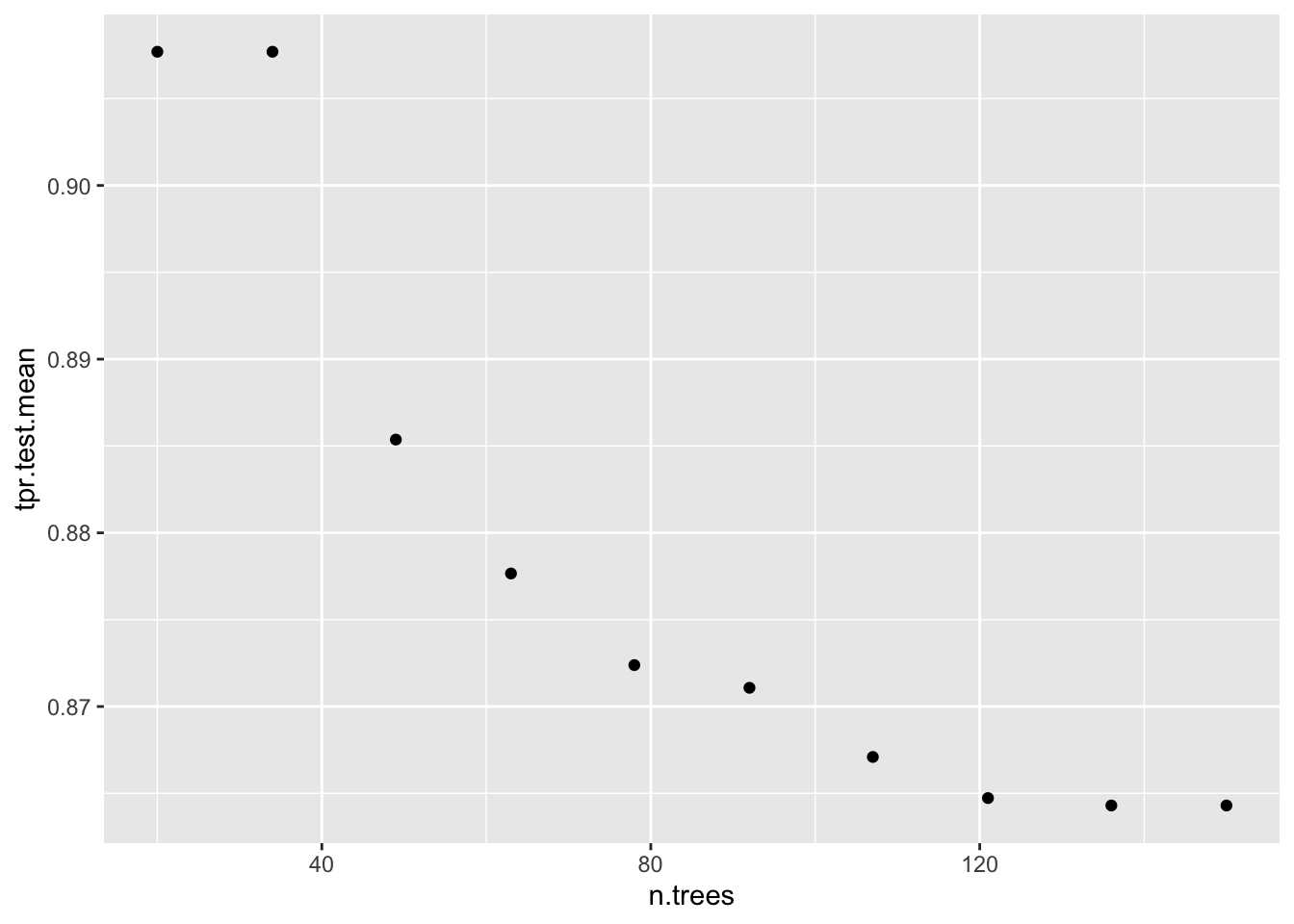
plotHyperParsEffect(data, x = "shrinkage", y = "tpr.test.mean", partial.dep.learn = makeLearner("regr.gbm"))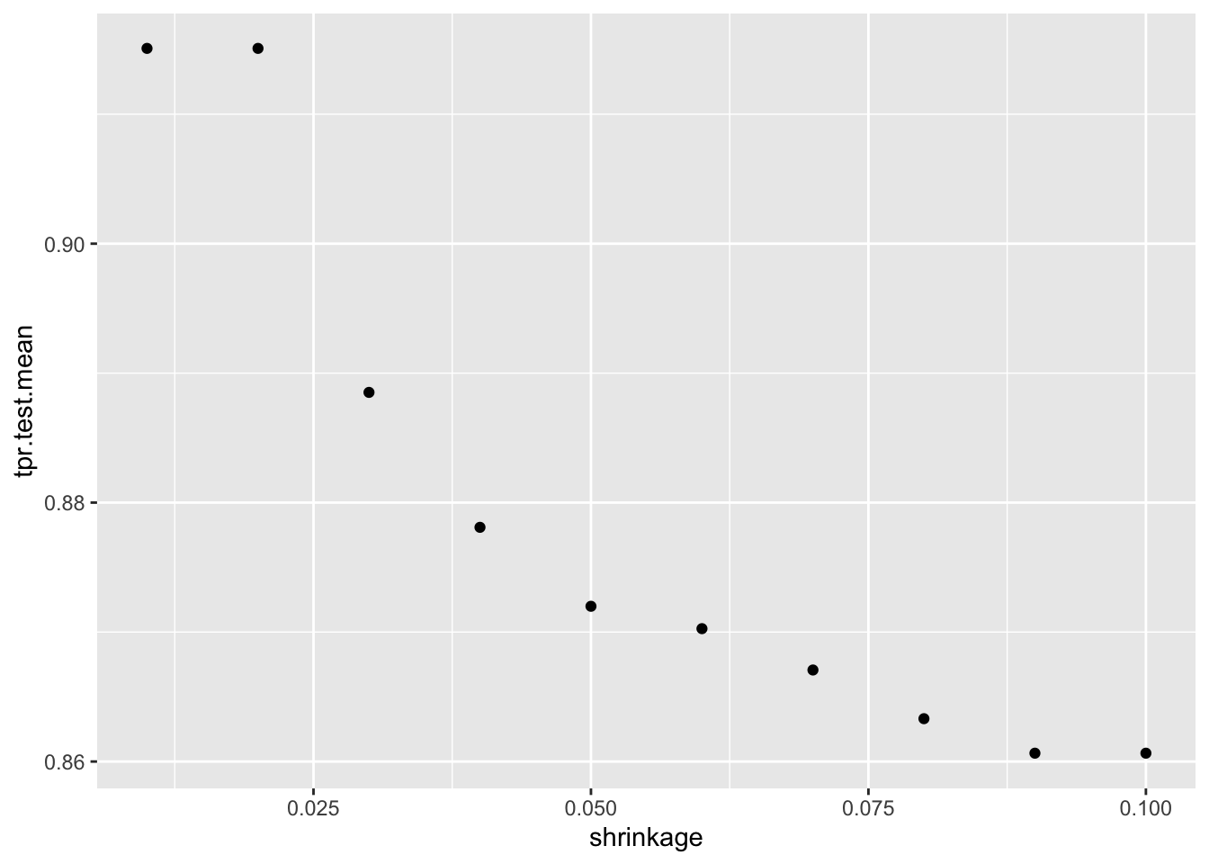
plotHyperParsEffect(data,
                    x = "n.trees",
                    y = "shrinkage",
                    z = "tpr.test.mean",
                    plot.type = "heatmap",
                    partial.dep.learn = makeLearner("regr.gbm")) +
  theme_bw() +
    labs(title = "Hyperparameter effects data",
         subtitle = "of GBM model with reduced feature set",
         caption = "Source: Pima Indians Diabetes Database")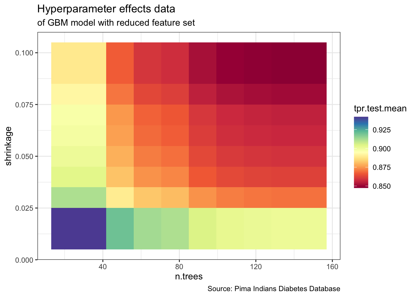
list( `Optimal HyperParameters` = dt_tuneparam$x,
      `Optimal Metrics` = dt_tuneparam$y )
## $`Optimal HyperParameters`
## $`Optimal HyperParameters`$n.trees
## [1] 20
##
## $`Optimal HyperParameters`$shrinkage
## [1] 0.02
##
##
## $`Optimal Metrics`
## tpr.test.mean auc.test.mean fnr.test.mean mmce.test.mean tnr.test.mean
## 1.0000000 0.7878691 0.0000000 0.3713375 0.0000000
## tpr.test.sd
## 0.0000000gbm_final <- setHyperPars(dt_prob, par.vals = dt_tuneparam$x)
set.seed(1000)
gbm_final_train <- train(learner = gbm_final, task = dt_task) ## Distribution not specified, assuming bernoulli ...getLearnerModel(gbm_final_train)## gbm::gbm(formula = f, data = d, n.trees = 20L, shrinkage = 0.02,
## keep.data = FALSE)
## A gradient boosted model with bernoulli loss function.
## 20 iterations were performed.
## There were 5 predictors of which 3 had non-zero influence.Decision Trees
- Recursive Partitioning (
rpart&rpart.plot)
library(rpart)
library(rpart.plot)

rpart_tree <- rpart(diabetes ~ .,
                    data = train,
                    method = "class")
rpart.plot(rpart_tree,
roundint=FALSE,
type = 3,
clip.right.labs = FALSE)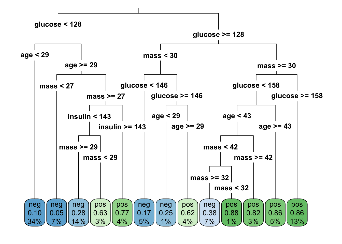
rpart.rules(rpart_tree, roundint = FALSE)## diabetes
## 0.05 when glucose < 128 & mass < 27 & age >= 29
## 0.10 when glucose < 128 & age < 29
## 0.17 when glucose is 128 to 146 & mass < 30
## 0.25 when glucose >= 146 & mass < 30 & age < 29
## 0.28 when glucose < 128 & mass >= 29 & age >= 29 & insulin < 143
## 0.38 when glucose is 128 to 158 & mass is 32 to 42 & age < 43
## 0.62 when glucose >= 146 & mass < 30 & age >= 29
## 0.63 when glucose < 128 & mass is 27 to 29 & age >= 29 & insulin < 143
## 0.77 when glucose < 128 & mass >= 27 & age >= 29 & insulin >= 143
## 0.82 when glucose is 128 to 158 & mass >= 42 & age < 43
## 0.86 when glucose is 128 to 158 & mass >= 30 & age >= 43
## 0.86 when glucose >= 158 & mass >= 30
## 0.88 when glucose is 128 to 158 & mass is 30 to 32 & age < 43Prediction
set.seed(1000)
(gbm_final_predict <- predict(gbm_final_train, newdata = test))
## Prediction: 154 observations
## predict.type: prob
## threshold: neg=0.50,pos=0.50
## time: 0.00
## truth prob.pos prob.neg response
## 12 pos 0.4807717 0.5192283 neg
## 18 pos 0.3229851 0.6770149 neg
## 19 neg 0.3229851 0.6770149 neg
## 20 pos 0.3300235 0.6699765 neg
## 34 neg 0.3091184 0.6908816 neg
## 38 pos 0.3229851 0.6770149 neg
## ... (#rows: 154, #cols: 4)gbm_final_predict %>% calculateROCMeasures()## predicted
## true neg pos
## neg 114 0 tpr: 1 fnr: 0
## pos 40 0 fpr: 1 tnr: 0
## ppv: 0.74 for: NaN lrp: 1 acc: 0.74
## fdr: 0.26 npv: NaN lrm: NaN dor: NaN
##
##
## Abbreviations:
## tpr - True positive rate (Sensitivity, Recall)
## fpr - False positive rate (Fall-out)
## fnr - False negative rate (Miss rate)
## tnr - True negative rate (Specificity)
## ppv - Positive predictive value (Precision)
## for - False omission rate
## lrp - Positive likelihood ratio (LR+)
## fdr - False discovery rate
## npv - Negative predictive value
## acc - Accuracy
## lrm - Negative likelihood ratio (LR-)
## dor - Diagnostic odds ratiomodel_performance <- performance(gbm_final_predict,
measures = list(tpr, auc, mmce, acc, tnr)) %>%
as.data.frame(row.names = c("True Positive Rate","Area Under Curve", "Mean Misclassification Error","Accuracy","True Negative Rate"))
model_performance## .
## True Positive Rate 1.0000000
## Area Under Curve 0.7695175
## Mean Misclassification Error 0.2597403
## Accuracy 0.7402597
## True Negative Rate 0.0000000gbm_final_threshold <- generateThreshVsPerfData(gbm_final_predict,
measures = list(tpr, auc, mmce, tnr))gbm_final_threshold %>%
plotROCCurves() +
geom_point() +
theme_bw() +
labs(title = "ROC curve from predictions",
subtitle = "of GBM model with reduced feature set",
caption = "Source: Pima Indians Diabetes Database")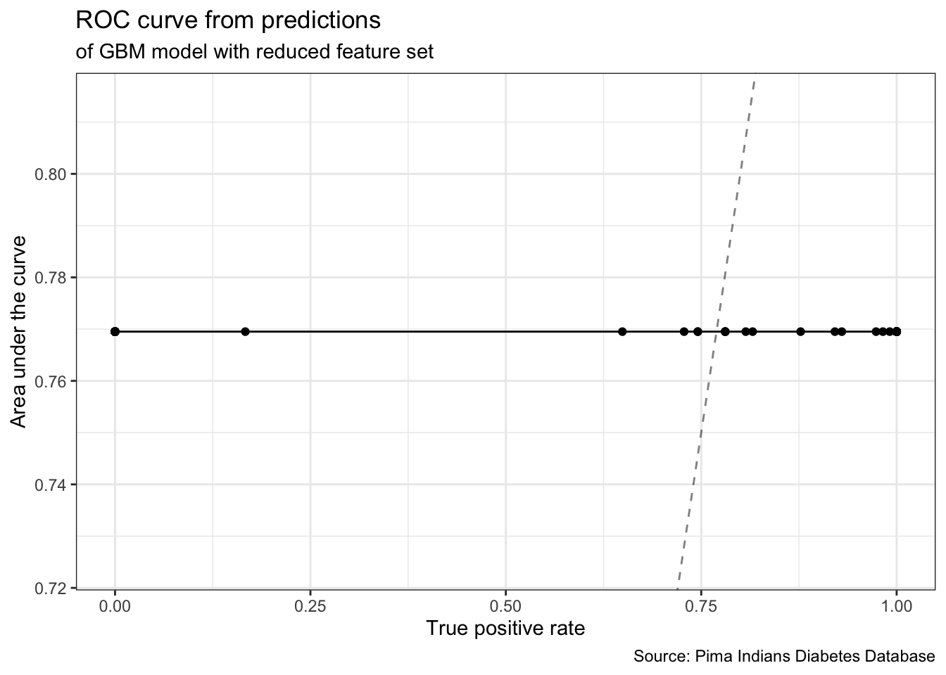
gbm_final_threshold %>%
   plotThreshVsPerf() +
   geom_point() +
    theme_bw() +
    labs(title = "Threshold vs. performance",
         subtitle = "for 2-class classification of GBM model with reduced feature set",
         caption = "Source: Pima Indians Diabetes Database")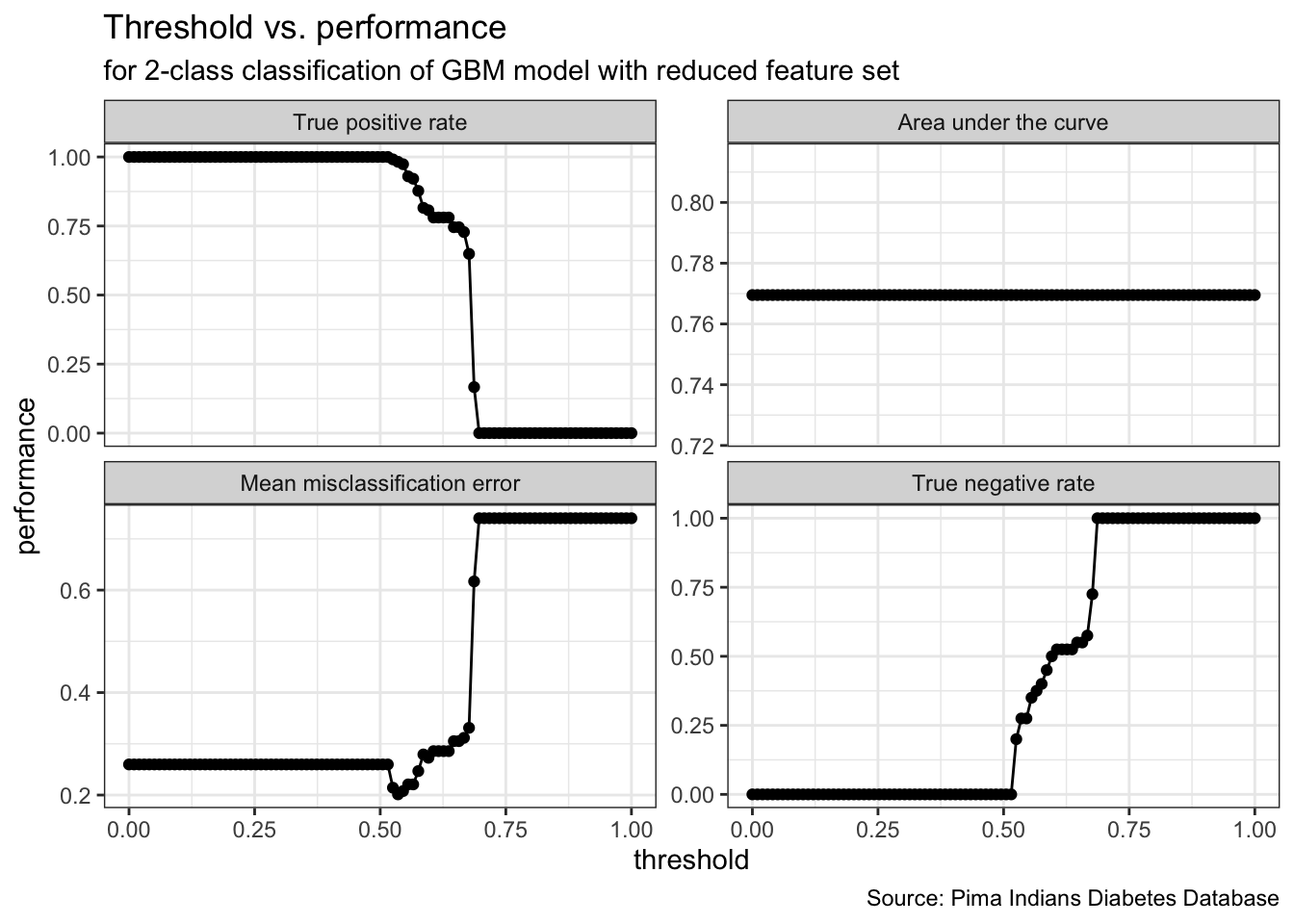
gbm_final_threshold$data %>%
  head()
## tpr auc mmce tnr threshold
## 1 1 0.7695175 0.2597403 0 0.00000000
## 2 1 0.7695175 0.2597403 0 0.01010101
## 3 1 0.7695175 0.2597403 0 0.02020202
## 4 1 0.7695175 0.2597403 0 0.03030303
## 5 1 0.7695175 0.2597403 0 0.04040404
## 6 1 0.7695175 0.2597403 0 0.05050505gbm_final_thr <- gbm_final_predict %>%
setThreshold(0.59595960)
(dt_performance <- gbm_final_thr %>% performance(measures = list(tpr, auc, mmce, tnr)) )## tpr auc mmce tnr
## 0.8070175 0.7695175 0.2727273 0.5000000(dt_cm <- gbm_final_thr %>% calculateROCMeasures() )## predicted
## true neg pos
## neg 92 22 tpr: 0.81 fnr: 0.19
## pos 20 20 fpr: 0.5 tnr: 0.5
## ppv: 0.82 for: 0.52 lrp: 1.61 acc: 0.73
## fdr: 0.18 npv: 0.48 lrm: 0.39 dor: 4.18
##
##
## Abbreviations:
## tpr - True positive rate (Sensitivity, Recall)
## fpr - False positive rate (Fall-out)
## fnr - False negative rate (Miss rate)
## tnr - True negative rate (Specificity)
## ppv - Positive predictive value (Precision)
## for - False omission rate
## lrp - Positive likelihood ratio (LR+)
## fdr - False discovery rate
## npv - Negative predictive value
## acc - Accuracy
## lrm - Negative likelihood ratio (LR-)
## dor - Diagnostic odds ratioperformance_threshold <- performance(gbm_final_thr, measures = list(tpr, auc, mmce, acc, tnr)) %>%
as.data.frame(row.names = c("True Positive Rate", "Area Under Curve", "Mean Misclassification Error", "Accuracy", "True Negative Rate"))
performance_threshold## .
## True Positive Rate 0.8070175
## Area Under Curve 0.7695175
## Mean Misclassification Error 0.2727273
## Accuracy 0.7272727
## True Negative Rate 0.5000000Decision Boundaries
#remotes::install_github("grantmcdermott/parttree")
library(parsnip)
library(parttree)
set.seed(123) ## For consistent jitter

## Build our tree using parsnip (but with rpart as the model engine)
ti_tree =
  decision_tree() %>%
  set_engine("rpart") %>%
  set_mode("classification") %>%
  fit(diabetes ~ glucose + mass, data = PimaIndiansDiabetes)

## Plot the data and model partitions
PimaIndiansDiabetes %>%
  ggplot(aes(x = glucose, y = mass)) +
  geom_jitter(aes(col = diabetes), alpha = 0.7) +
  geom_parttree(data = ti_tree, aes(fill = diabetes), alpha = 0.1) +
  theme_bw() +
    labs(title = "Decision boundaries",
         subtitle = "for 2-class classification of RPART model (glucose + mass)",
         caption = "Source: Pima Indians Diabetes Database")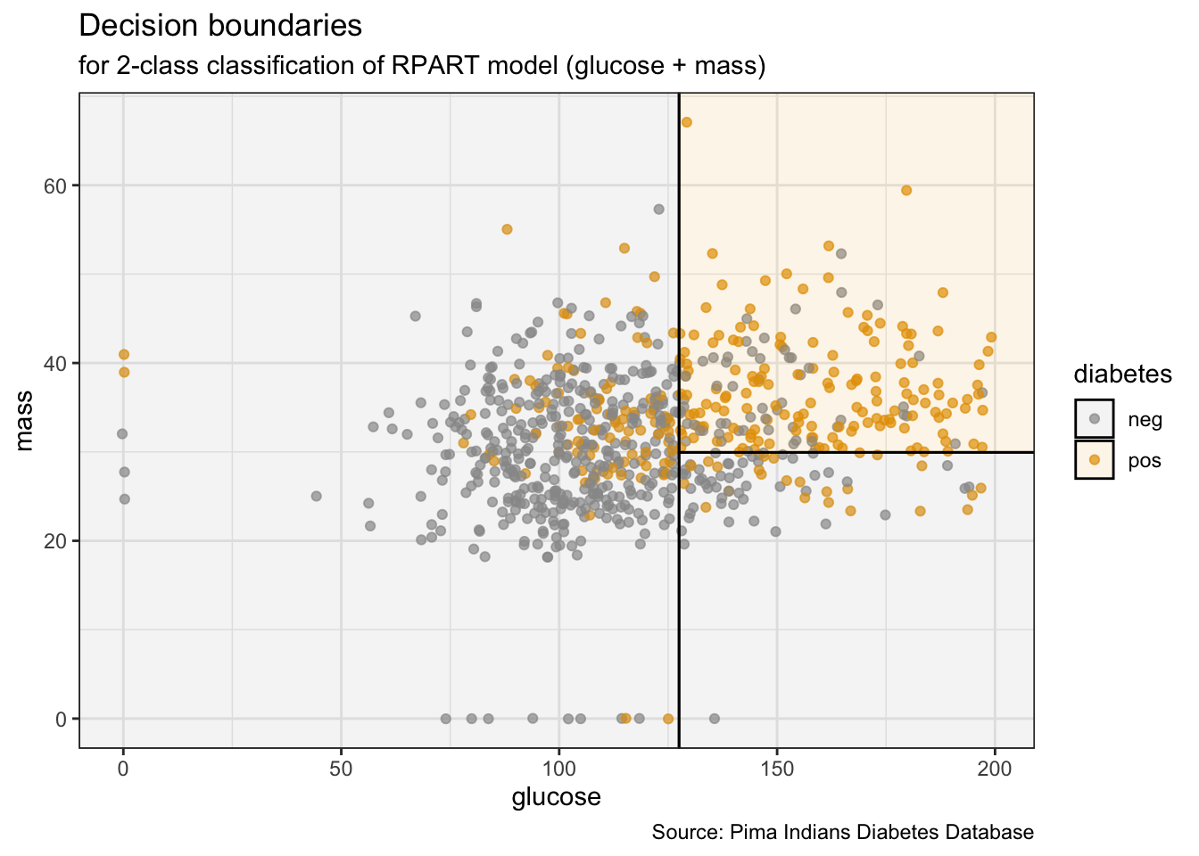
Time-series
Artificial Neural Networks (ANNs)
Li et al, Visualizing the Loss Landscape of Neural Nets, 2018
Visualizing Data using the Embedding Projector in TensorBoard
Visualizing and Understanding Convolutional Networks, Zeiler & Fergus, 2013
Play with Generative Adversarial Networks (GANs) in your browser
Whose dream is this? When and how to use the Keras Functional API
 - Deep Learning with Keras and TensorFlow & Update with TF 2.0: Image classification with Keras and TensorFlow
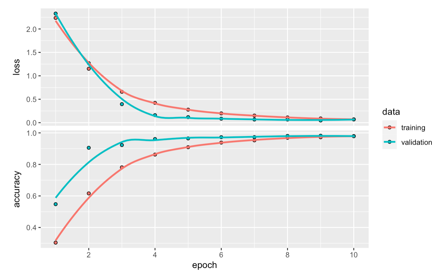
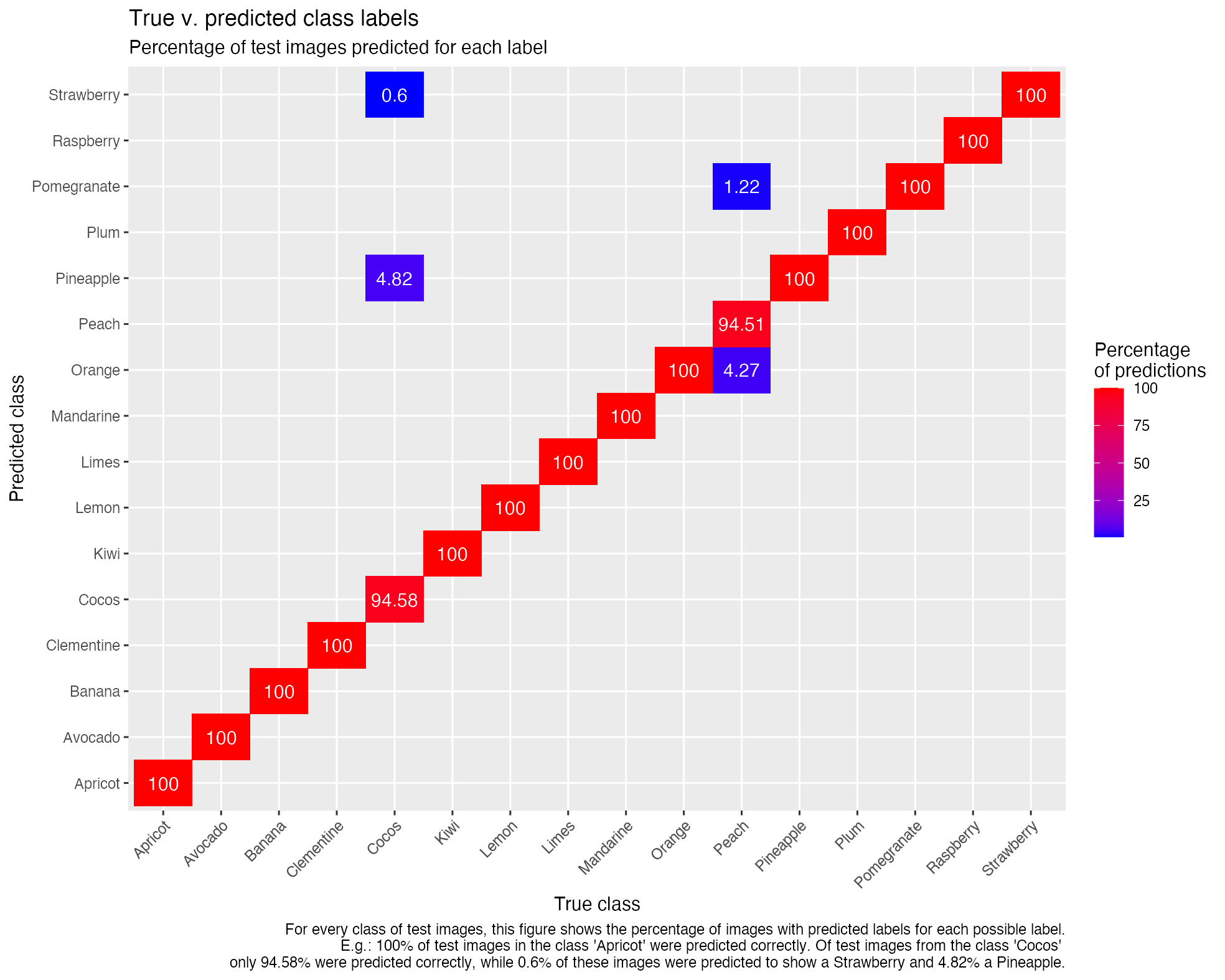
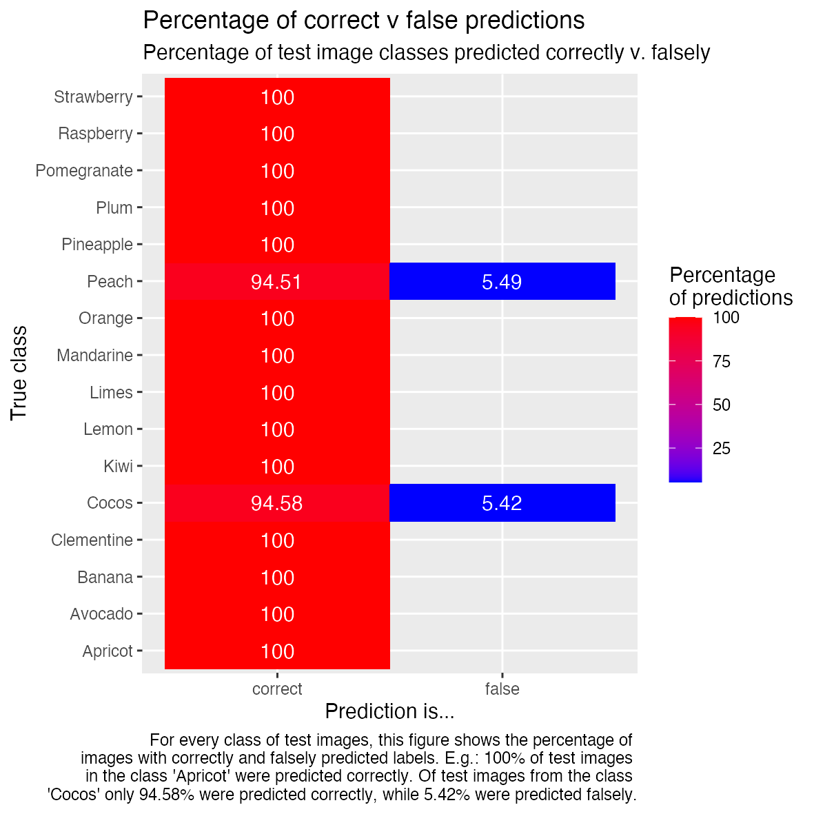
Graphical representation of a model in TensorBoard
Word Embeddings
Explainable AI
# session info
devtools::session_info()
## ─ Session info ───────────────────────────────────────────────────────────────
## setting value
## version R version 4.0.4 (2021-02-15)
## os macOS Big Sur 10.16
## system x86_64, darwin17.0
## ui X11
## language (EN)
## collate en_US.UTF-8
## ctype en_US.UTF-8
## tz Europe/Berlin
## date 2021-04-27
##
## ─ Packages ───────────────────────────────────────────────────────────────────
## package * version date lib
## assertthat 0.2.1 2019-03-21 [2]
## backports 1.2.1 2020-12-09 [2]
## BBmisc 1.11 2017-03-10 [2]
## blogdown 1.2 2021-03-04 [2]
## bookdown 0.21 2020-10-13 [2]
## broom 0.7.5 2021-02-19 [2]
## bslib 0.2.4 2021-01-25 [2]
## cachem 1.0.4 2021-02-13 [2]
## callr 3.5.1 2020-10-13 [2]
## cellranger 1.1.0 2016-07-27 [2]
## checkmate 2.0.0 2020-02-06 [2]
## cli 2.3.1 2021-02-23 [2]
## colorspace 2.0-0 2020-11-11 [2]
## crayon 1.4.1 2021-02-08 [2]
## data.table 1.14.0 2021-02-21 [2]
## DBI 1.1.1 2021-01-15 [2]
## dbplyr 2.1.0 2021-02-03 [2]
## desc 1.3.0 2021-03-05 [2]
## devtools 2.3.2 2020-09-18 [2]
## digest 0.6.27 2020-10-24 [2]
## dplyr * 1.0.5 2021-03-05 [2]
## ellipsis 0.3.1 2020-05-15 [2]
## entropy 1.2.1 2014-11-14 [1]
## evaluate 0.14 2019-05-28 [2]
## fansi 0.4.2 2021-01-15 [2]
## farver 2.1.0 2021-02-28 [2]
## fastmap 1.1.0 2021-01-25 [2]
## fastmatch 1.1-0 2017-01-28 [2]
## forcats * 0.5.1 2021-01-27 [2]
## fs 1.5.0 2020-07-31 [2]
## FSelector * 0.33 2021-02-16 [1]
## gbm 2.1.8 2020-07-15 [2]
## generics 0.1.0 2020-10-31 [2]
## GGally * 2.1.1 2021-03-08 [1]
## ggfortify * 0.4.11 2020-10-02 [2]
## ggplot2 * 3.3.3 2020-12-30 [2]
## glue 1.4.2 2020-08-27 [2]
## gridExtra 2.3 2017-09-09 [2]
## gtable 0.3.0 2019-03-25 [2]
## haven 2.3.1 2020-06-01 [2]
## highr 0.8 2019-03-20 [2]
## hms 1.0.0 2021-01-13 [2]
## htmltools 0.5.1.1 2021-01-22 [2]
## httr 1.4.2 2020-07-20 [2]
## jquerylib 0.1.3 2020-12-17 [2]
## jsonlite 1.7.2 2020-12-09 [2]
## knitr 1.31 2021-01-27 [2]
## labeling 0.4.2 2020-10-20 [2]
## lattice 0.20-41 2020-04-02 [2]
## lifecycle 1.0.0 2021-02-15 [2]
## lubridate 1.7.10 2021-02-26 [2]
## magrittr 2.0.1 2020-11-17 [2]
## MASS * 7.3-53.1 2021-02-12 [2]
## Matrix 1.3-2 2021-01-06 [2]
## memoise 2.0.0 2021-01-26 [2]
## mlbench * 2.1-3 2021-01-29 [1]
## mlr * 2.19.0 2021-02-22 [2]
## mmpf * 0.0.5 2018-10-24 [2]
## modelr 0.1.8 2020-05-19 [2]
## munsell 0.5.0 2018-06-12 [2]
## parallelMap 1.5.0 2020-03-26 [2]
## ParamHelpers * 1.14 2020-03-24 [2]
## parsnip * 0.1.5 2021-01-19 [2]
## parttree * 0.0.1.9000 2021-03-14 [1]
## pillar 1.5.1 2021-03-05 [2]
## pkgbuild 1.2.0 2020-12-15 [2]
## pkgconfig 2.0.3 2019-09-22 [2]
## pkgload 1.2.0 2021-02-23 [2]
## plyr 1.8.6 2020-03-03 [2]
## prettyunits 1.1.1 2020-01-24 [2]
## processx 3.4.5 2020-11-30 [2]
## ps 1.6.0 2021-02-28 [2]
## purrr * 0.3.4 2020-04-17 [2]
## R6 2.5.0 2020-10-28 [2]
## randomForest 4.6-14 2018-03-25 [2]
## RColorBrewer 1.1-2 2014-12-07 [2]
## Rcpp 1.0.6 2021-01-15 [2]
## readr * 1.4.0 2020-10-05 [2]
## readxl 1.3.1 2019-03-13 [1]
## remotes 2.2.0 2020-07-21 [2]
## reprex 1.0.0 2021-01-27 [2]
## reshape 0.8.8 2018-10-23 [1]
## rJava * 0.9-13 2020-07-06 [2]
## rlang 0.4.10 2020-12-30 [2]
## rmarkdown 2.7 2021-02-19 [2]
## rpart * 4.1-15 2019-04-12 [2]
## rpart.plot * 3.0.9 2020-09-17 [1]
## rprojroot 2.0.2 2020-11-15 [2]
## rstudioapi 0.13 2020-11-12 [2]
## rvest 1.0.0 2021-03-09 [2]
## RWeka 0.4-43 2020-08-23 [1]
## RWekajars 3.9.3-2 2019-10-19 [1]
## sass 0.3.1 2021-01-24 [2]
## scagnostics * 0.2-4.1 2018-04-04 [1]
## scales 1.1.1 2020-05-11 [2]
## sessioninfo 1.1.1 2018-11-05 [2]
## stringi 1.5.3 2020-09-09 [2]
## stringr * 1.4.0 2019-02-10 [2]
## survival 3.2-7 2020-09-28 [2]
## testthat 3.0.2 2021-02-14 [2]
## tibble * 3.1.0 2021-02-25 [2]
## tidyr * 1.1.3 2021-03-03 [2]
## tidyselect 1.1.0 2020-05-11 [2]
## tidyverse * 1.3.0 2019-11-21 [2]
## usethis 2.0.1 2021-02-10 [2]
## utf8 1.2.1 2021-03-12 [2]
## vctrs 0.3.6 2020-12-17 [2]
## withr 2.4.1 2021-01-26 [2]
## xfun 0.22 2021-03-11 [2]
## XML 3.99-0.5 2020-07-23 [2]
## xml2 1.3.2 2020-04-23 [2]
## yaml 2.2.1 2020-02-01 [2]
## source
## CRAN (R 4.0.0)
## CRAN (R 4.0.2)
## CRAN (R 4.0.2)
## CRAN (R 4.0.2)
## CRAN (R 4.0.2)
## CRAN (R 4.0.4)
## CRAN (R 4.0.2)
## CRAN (R 4.0.2)
## CRAN (R 4.0.2)
## CRAN (R 4.0.0)
## CRAN (R 4.0.2)
## CRAN (R 4.0.4)
## CRAN (R 4.0.2)
## CRAN (R 4.0.2)
## CRAN (R 4.0.4)
## CRAN (R 4.0.2)
## CRAN (R 4.0.2)
## CRAN (R 4.0.2)
## CRAN (R 4.0.2)
## CRAN (R 4.0.2)
## CRAN (R 4.0.2)
## CRAN (R 4.0.0)
## CRAN (R 4.0.2)
## CRAN (R 4.0.1)
## CRAN (R 4.0.2)
## CRAN (R 4.0.2)
## CRAN (R 4.0.2)
## CRAN (R 4.0.2)
## CRAN (R 4.0.2)
## CRAN (R 4.0.2)
## CRAN (R 4.0.2)
## CRAN (R 4.0.2)
## CRAN (R 4.0.2)
## CRAN (R 4.0.2)
## CRAN (R 4.0.2)
## CRAN (R 4.0.2)
## CRAN (R 4.0.2)
## CRAN (R 4.0.2)
## CRAN (R 4.0.0)
## CRAN (R 4.0.2)
## CRAN (R 4.0.0)
## CRAN (R 4.0.2)
## CRAN (R 4.0.2)
## CRAN (R 4.0.2)
## CRAN (R 4.0.2)
## CRAN (R 4.0.2)
## CRAN (R 4.0.2)
## CRAN (R 4.0.2)
## CRAN (R 4.0.4)
## CRAN (R 4.0.2)
## CRAN (R 4.0.2)
## CRAN (R 4.0.2)
## CRAN (R 4.0.2)
## CRAN (R 4.0.4)
## CRAN (R 4.0.2)
## CRAN (R 4.0.2)
## CRAN (R 4.0.4)
## CRAN (R 4.0.2)
## CRAN (R 4.0.2)
## CRAN (R 4.0.0)
## CRAN (R 4.0.2)
## CRAN (R 4.0.2)
## CRAN (R 4.0.2)
## Github (grantmcdermott/parttree@9d25d2c)
## CRAN (R 4.0.2)
## CRAN (R 4.0.2)
## CRAN (R 4.0.0)
## CRAN (R 4.0.4)
## CRAN (R 4.0.0)
## CRAN (R 4.0.0)
## CRAN (R 4.0.2)
## CRAN (R 4.0.2)
## CRAN (R 4.0.0)
## CRAN (R 4.0.2)
## CRAN (R 4.0.2)
## CRAN (R 4.0.0)
## CRAN (R 4.0.2)
## CRAN (R 4.0.2)
## CRAN (R 4.0.2)
## CRAN (R 4.0.2)
## CRAN (R 4.0.2)
## CRAN (R 4.0.2)
## CRAN (R 4.0.2)
## CRAN (R 4.0.2)
## CRAN (R 4.0.4)
## CRAN (R 4.0.4)
## CRAN (R 4.0.2)
## CRAN (R 4.0.2)
## CRAN (R 4.0.2)
## CRAN (R 4.0.2)
## CRAN (R 4.0.2)
## CRAN (R 4.0.2)
## CRAN (R 4.0.2)
## CRAN (R 4.0.2)
## CRAN (R 4.0.0)
## CRAN (R 4.0.0)
## CRAN (R 4.0.2)
## CRAN (R 4.0.0)
## CRAN (R 4.0.4)
## CRAN (R 4.0.2)
## CRAN (R 4.0.2)
## CRAN (R 4.0.2)
## CRAN (R 4.0.0)
## CRAN (R 4.0.0)
## CRAN (R 4.0.2)
## CRAN (R 4.0.4)
## CRAN (R 4.0.2)
## CRAN (R 4.0.2)
## CRAN (R 4.0.2)
## CRAN (R 4.0.2)
## CRAN (R 4.0.0)
## CRAN (R 4.0.0)
##
## [1] /Users/shiringlander/Library/R/4.0/library
## [2] /Library/Frameworks/R.framework/Versions/4.0/Resources/library
